Munich Personal RePEc Archive
Modelling Stock Return Volatility in
India
Kumari, Sujata and Sahu, Priyanka
University of Hyderabad
10 March 2018
Modelling Stock Return Volatilities in India
ABSTRACT
This paper empirically estimates the clustering volatility of the Indian stock market by
considering twelve indicators of BSE SENSEX. The cluster volatility has been estimated
through ARCH family models such as ARCH, GARCH, IGARCH, GARCH-M, EGARCH,
TARCH, GJR TARCH, SAARCH, PARCH, NARCH, NARCHK, APARCH, and NPARCH.
KEYWORDS: Clustering Volatility, BSE SENSEX, ARCH Effects, asymmetric information.
Section -1
1.1. INTRODUCTION
Volatility is defined as the conditional heteroscedasticity, which explains the conditional
standard deviations of the underlying asset return. It is an important factor in trading system in
the stock market. Volatility has various application in financial institutions. In the modern
financial econometrics, the ARCH (Autoregressive Conditional Heteroscedasticity) model was
introduced by Engel (1982). It has been observed that stock market volatility changes with
time or we can say that it is time – varying and exhibits volatility clustering, which is nothing but the variance (standard deviation) measures as the risk and elements of uncertainty.
Volatility changes occur because of time – varying, which requires more empirical estimation of financial time series over the period of time. In financial time series analysis, all the
statistical theory and methods plays an important role. There are specials features which tells
about the volatility of stock return, which is not directly observable.
There are certain characteristics that are common in asset returns. Firstly, it has a volatility
clusters, it means that volatility may be high for the certain period and low for the others
periods. Secondly, volatility evolves over time in a continuous manner. Thirdly, volatility doesn’t diverge to infinity that is volatility varies within a fixed range. Fourthly, volatility seems to react in a different manner to a big price increase or a big price drop, that is called as
leverage effect.
The rest of the paper is follows as; introduction is followed by literature review in section 2
well as empirical studies. Section 3 and 4, discuss the empirical estimation and findings and
conclusion.
Section II- Literature Review
2.1. Theoretical Modelling
The univariate volatility models, which is discussed in the paper are the autoregressive
conditional heteroscedastic (ARCH) model of Engel (1982) , the generalized ARCH (GARCH)
model of Bollerslev (1986) the Integrated GARCH (1990) and exponential GARCH
(EGARCH ) model of Nelson (1991) Threshold ARCH (TARCH) model of Zakoian (1994) ,
GJR , from threshold ARCH Glosten , Jagannathan and Runkel (1993) , Simple Asymmetric
ARCH (SAARCH) model( 1990 ) of Engel, Power ARCH ( PARCH) model ( 1992) of Higgins
and Bera, Nonlinear ARCH (NARCH) model, Nonlinear with one shift ( NARCHK)
Asymmetric power ARCH ( APARCH) model (1993) of Ding , Granger and Engel and the last
model is Nonlinear power ARCH ( NPARCH) model .
Structure of a Model
Let’s consider mean and variance of 𝑟𝑡 is given as;
𝜇𝑡 = E(𝑟𝑡⁄𝐹𝑡−1) and E [(𝑟𝑡− 𝜇𝑡)2⁄𝐹𝑡−1]
𝜎𝑡2 = var (𝑟𝑡⁄𝐹𝑡−1) (1)
Where,
𝐹𝑡−1 denotes the information set available at one lag period. Typically, 𝐹𝑡−1 consists of
all linear function of the past returns. Here, 𝑟𝑡 follows a simple time series model such as
stationary ARMA ( p , q ) model with explanatory variables and shocks or error terms. In other
words, we entertain the model as;
𝑟𝑡 = 𝜇𝑡 + 𝑎𝑡 ,
Where, 𝜇𝑡 = ∅0 + ∑𝑘𝑖=1𝛽𝑖𝑥𝑖𝑡 + ∑𝑃𝑖=1∅𝑖𝑟𝑡−1 - ∑𝑞𝑖=1𝜃𝑖𝑎𝑡−𝑖 (2)
Equation (2) illustrates the financial application of the time series model, where k ,p , q are
non – negative integers and 𝑥𝑖𝑡 is the explanatory variables . The explanatory variables 𝑥𝑡 in
equation (2) are flexible. We can take an example about the daily returns of market index,
which often shows serial correlation and if we talk about monthly returns of markets index
Combining equation (1) and (2), we have
𝜎𝑡2 = var (𝑟𝑡 𝐹
𝑡−1
⁄ ) = var (𝑎𝑡 𝐹
𝑡−1
⁄ ) (3)
The conditional heteroscedastic model is concerned with the evolution of 𝜎𝑡2 . The manner
under which 𝜎𝑡2 evolves over time distinguishes one volatility model from another. Where, 𝑎𝑡
is the shock or innovation of an asset return at time t and 𝜎𝑡 is the positive square root of 𝜎𝑡2.
Therefore, modelling conditional heteroscedasticity, explains the time evolution of the
conditional variance of an asset return. This paper discusses the modelling of the volatility of
stock return with the following time series models, is discussed as below.
1. Arch Model
Autoregressive conditional heteroscedasticity (ARCH) model was introduced by Engel (1982)
that provides a systematic framework for volatility modelling. The basic idea of ARCH model
is that (a) the stock 𝑎𝑡of an asset return should be serially uncorrelated and (b) the dependence
of 𝑎𝑡 can be shown by a simple quadratic function with its lagged values . Specifically, an
ARCH (m) model take the form as,
𝑎𝑡 = 𝜎𝑡𝜖𝑡 , 𝜎𝑡2 = 𝛼0 + 𝛼1𝑎𝑡−12 + --- + 𝛼𝑚𝑎𝑡−𝑚2 (4)
Where,
{𝜖𝑡} is a sequence of independent and identically distributed random variables with mean zero
and variance constant and where, 𝛼0 > 0. The coefficients of the regressors must satisfy some
regularity conditions to ensure that the unconditional variance of 𝑎𝑡 is finite. 𝜖𝑡 is assumed to
follow the standard normal or a standardized student t- distribution or a generalized error
distribution. From the structure of the model, it is seen that large past squared shocks imply a
large conditional variance 𝜎𝑡2 for the innovation 𝑎𝑡, which means that , under the ARCH model
framework , large shocks tend to be followed by another large shocks . This features are similar to the volatility clustering’s observed in asset returns.
Properties of Arch Model
First , the unconditional mean of 𝑎𝑡 remains zero because
𝐸(𝑎𝑡) = E [𝐸 (𝑎𝑡 𝐹
𝑡−1
⁄ )] = E[𝜎𝑡𝐸(𝜖𝑡)] = 0
Var (𝑎𝑡) = E (𝑎𝑡2) = E [𝐸 (𝑎𝑡2 𝐹
𝑡−1
⁄ )] = E (𝛼0+ 𝛼1𝑎𝑡−12) = 𝛼0+ 𝛼1𝐸(𝑎𝑡−12), is a
stationary process.
2. Garch Model
Bollerslev (1986) proposes this model, which is an extension of ARCH model popularly
known as the generalized ARCH (GARCH).
For a log return series 𝑟𝑡 , let 𝑎𝑡 = 𝑟𝑡 − 𝜇𝑡 be the innovation at time t . Then 𝑎𝑡 follows a
GARCH (m ,s ) model IGARC
If 𝑎𝑡 = 𝜎𝑡𝜖𝑡 , 𝜎𝑡2 = 𝛼0 + ∑𝑚𝑖=1𝛼𝑖𝑎𝑡−𝑖2+ ∑𝑠𝑗=1𝛽𝑗𝜎𝑡−𝑗2 (5)
where,
{𝜖𝑡} is a sequence of independent and identity distributed random variables with mean
zero and variance constant. Here, 𝛼𝑖 = 0 for i > m and 𝛽𝑗 = 0 for j > s . We observed that the
constraint on 𝛼𝑖 + 𝛽𝑖 shows that the unconditional variance of 𝑎𝑡 is finite, where as its
conditional variance 𝜎𝑡2 evolves overtime. 𝜖𝑡 is often assumed to be a standard normal or
standardized student – t distribution or generalized error distribution.
The strength and weaknesses of GARCH models can be easily seen by focusing on the
simplest GARCH model with
𝜎𝑡2 = 𝛼0 + 𝛼1𝑎𝑡−12+ 𝛽1𝜎𝑡−12
where, α1 ≤ 0, β1 ≤ 1 and (α1+ β1) < 1 (7)
This model investigates the weaknesses of the ARCH Model. It follows both positive and
negative shocks.
3. The Integrated Garch Model
𝑎𝑡2 = 𝛼0 + ∑max(𝑚 ,𝑠)𝑖=1 (𝛼𝑖 + 𝛽𝑖) 𝑎𝑡2+ ᵑ𝑡− ∑𝑠𝑗=1𝛽𝑗ᵑ𝑡−𝑗 (8)
Above equation is the AR polynomial GARCH representation, has unit root, also represented
as unit root IGARCH models. It is similar to ARIMA model ,the key feature of IGARCH
models is that the impact of past squared shocks 𝜂𝑡−𝑖 = 𝑎𝑡−𝑖2− 𝜎𝑡−𝑖2 𝑓𝑜𝑟 𝑖 >
0 𝑜𝑛 𝑎𝑡2 is persistent.
𝑎𝑡 = 𝜎𝑡𝜖𝑡 , 𝜎𝑡2 = 𝛼0+ 𝛽1𝜎𝑡−12 + (1 − 𝛽1) 𝑎𝑡−12 (9)
The unconditional variance of 𝑎𝑡 is not defined under the above IGARCH model .It is difficult
to justify for an excess return series . From a theoretical point of view, the IGARCH
phenomenon has been caused by occasional level shifts in volatility. Exponential smoothing
methods which is used to estimate such an IGARCH model.
4. The Garch-M Model
GARCH-M, where “M” stand for GARCH in mean. A simple GARCH – M model can be written as
𝑟𝑡 = 𝜇 + 𝐶𝜎𝑡2 + 𝑎𝑡 , 𝑎𝑡 = 𝜎𝑡𝜖𝑡
𝜎𝑡2 = 𝛼0 + 𝛼1𝑎𝑡−12+ 𝛽1𝜎𝑡−12 , (10)
Where
, μ and C are constants . The parameter C is called the risk premium parameter.Positive C indicates that the return is positively related to its volatility.
5. The exponential GARCH (EGARCH) model
This EGARCH model was introduced by Nelson (1991), this Exponential GARCH model explains that asymmetric effects between positive and negative of asset returns.
𝑔(𝜖𝑡) = 𝜃𝜖𝑡+ 𝛾[⃓𝜖𝑡⃓− 𝐸(⃓𝜖𝑡⃓)] , (11)
Where 𝜃 𝑎𝑛𝑑 𝛾 𝑎𝑟𝑒 𝑑𝑒𝑛𝑜𝑡𝑒𝑑 𝑎𝑠 𝑟𝑒𝑎𝑙 𝑐𝑜𝑛𝑠𝑡𝑎𝑛𝑡𝑠 . 𝐵𝑜𝑡ℎ 𝜖𝑡 𝑎𝑛𝑑 ⃓𝜖𝑡⃓ − 𝐸(⃓𝜖𝑡⃓) 𝑎𝑟𝑒 𝑧𝑒𝑟𝑜
mean iid sequence with continuous distributions . Therefore , E [𝑔(𝜖𝑡)] = 0 . The asymmetry
of [𝑔(𝜖𝑡)] can easily be shown by rewriting it as
𝑔𝜖𝑡 = {(𝜃 + 𝛾) 𝜖𝑡 − 𝛾𝐸 (⃓𝜖𝑡⃓) 𝑖𝑓 𝜖𝑡 ≥ 0
(𝜃 − 𝛾)𝜖𝑡− 𝛾𝐸 (⃓𝜖𝑡⃓) < 0
6. THE THRESOLD GARCH (TGARCH) model
TGARCH model was developed by Zakoian (1994), Glosten , Jagannathan and Runkle (1993). TGARCH ( m , s )model takes the form as;
𝜎𝑡2 = 𝛼0+ ∑ (𝛼𝑠𝑖=1 𝑖 + 𝛾𝑖𝑁𝑡−𝑖)𝑎𝑡−𝑖2+ ∑𝑚𝑗−1𝛽𝑗𝜎𝑡−𝑗2 (12)
Where , 𝑁𝑡−𝑖 is an indicate for negative 𝑎𝑡−𝑖 , that is , 𝑁𝑡−𝑖 = { 1 𝑖𝑓𝑎𝑡−𝑖 < 0 ,
and 𝛼𝑖, 𝛾𝑖 , 𝑎𝑛𝑑 𝛽𝑗 are known as non-negative parameters , which is satisfying conditions as
similar to those of GARCH models . From this model , we observed that a positive 𝑎𝑡−1
contributes 𝛼𝑖𝑎𝑡−𝑖2 𝑡𝑜 𝜎𝑡2, 𝑤ℎ𝑒𝑟𝑒 𝑎 𝑛𝑒𝑔𝑎𝑡𝑖𝑣𝑒 𝑎𝑡−𝑖 has a larger impact (𝛼𝑖+ 𝛾𝑖) + 𝑎𝑡−𝑖2
with 𝛾𝑖 > 0 . This model uses zero as its Threshold
7. GJR Form of Threshold Garch Model
This model GJR- TGARCH was framed by Glosten, Jagannathan and Runkle (1993) which relaxed the restrictions of conditional variance dynamics. Above equation (12) shows
the same. where 𝑟𝑡 is the series of demeaned returns and 𝜎𝑡2 is the conditional variance of
returns given time t information . We assume that the sequence of innovations 𝜖𝑡 follow
independent and identical distribution with mean 0 and variance 1: 𝜖𝑡 ∼ iidD (0, 1) .
GJR-TGARCH reveals leverage effect which is that good news has an impact on volatility greater
than bad news.
8. Simple Asymmetric ARCH model
This (SAARCH) simple asymmetric ARCH model (1990) of Granger Engel, which follows above two models, such as –(EGARCH) Exponential GARCH model of Nelson (1991)
and (TGARCH) and GJR-TGARCH model by Zakoian (1994), Glosten, Jagannathan and
Runkle (1993) and power GARCH (PGARCH) model. These models are describing the
asymmetric volatility process. This characteristic in the financial market has become known as “Leverageeffects “. Which is actually meaning is that it follows the symmetric response of volatility negative and positive shocks, this is the primary restrictions of GARCH model. In
this model a negative sock in the financial time series, that is the cause of volatility to increase
the positive shocks in the same magnitude. Basically it shows the relationship between
asymmetric volatility and return.
9. Power arch (parch) model
This model PARCH was given by Higgins and Bera (1992). Nelson (1990a, b) and Gannon (1996) have reformed the relationship between the estimation of ARCH models and
the identification of the mean equation. Their general conclusion drawn from their work i.e.,
the identification of the mean equation creates small impact on the ARCH model when it’s estimated in continuous time. In the mean equation should be identified as an expected mean
reverting equation in the form of 𝑟𝑡 = 𝜖𝑡 "t where , 𝑟𝑡 is the returns to the market index. This
variance of one . The general power ARCH model introduced by Ding et al. (1993), identifies
𝜎𝑡 as a form ,
𝜎𝑡𝑑 = 𝛼0+ ∑ 𝛼𝑝𝑡−𝑖 𝑖(|𝜖𝑡−1| + 𝛾𝑖𝜖𝑡−𝑖)𝑑+ ∑𝑞𝑖=1𝛽𝑖𝜎𝑡−𝑖𝑑 (13)
Where , in the above equation ( 13 ) shows as 𝛼𝑖 𝑎𝑛𝑑 𝛽𝑖 called as the standard ARCH and
GARCH parameters , 𝛾𝑖 is the leverage parameter and d is the parameter for the power term.
10. Nonlinear arch (narch) model
Non-linear ARCH ( NARCH) model was also developed by Higgins and Bera ( 1990) ,which was obtained same as the above PARCH model equation ( 13 ) , shows that d and 𝛼𝑖
are free ( 𝛼𝑖 = 0 , 𝛽𝑖 = 0 ) . If this NARCH model allows to free to 𝛽𝑖 is equal to zero then
the PGARCH will give specified is the results .
11. Nonlinear arch with one shift model
It is also called as NARCHK , which means that there is specifying lags between two parameters term, such as 𝛼𝑖(𝜖𝑡− 𝑘)2 this is nothing as the variations of the nonlinear arch model , where ‘ k ‘ is constant for all lags . there is difference between two models NARCH and NARCH with one shift, which tells about past lags. It is not collinear with other models
ARCH, SAARCH, NARCH, NAPARCHK and NAPARCH.
12. Asymmetric power arch (aparch) model
This model was decorated by Ding, Granger, Engle (1993), identified the generalise asymmetric Power ARCH model, in financial time series this model plays important role for
stock market. The important purpose of this model is that to identified the variance of error
term in a regression equation, of its square past errors. This APARCH model satisfies in the
above given model PARCH and its equation (13), restrictions is to require to produce for each
of the models, which given within APARCH model. The power term provided by this model
which is generated above given models NARCH, PARCH and APARCH. This term
asymmetric which is include in generated Ding et al power ARCH models, which measuring
all the positive and negative in equal magnitude shocks of the return in the financial markets.
13. Nonlinear power arch (nparch) model
This also measures the asymmetric impacts on shocks or innovations in a specified form
lagged innovations or shocks are all zero, and on the other hand that the symmetric response to
lagged innovations or shocks but all are not zero. If there is conditional variance is small, then
there is no “NO NEWS ARE GOODS NEWS “. This model as similar to others models, NARCH, NARCHK, NPARCH. All these models have responded the symmetric innovations.
There is minimum variance which lies at positive and negative value for innovations or shocks.
2.2. Empirical reviews of literature
There is literature based on modelling and measuring stock return volatilities in India. Ahmed
et al. (2011) investigated the volatility using daily data from two Middle East stock indices
viz., the Egyptian cma index and the Israeli tase-100 index and used ARCH, GARCH,
EGARCH, TGARCH, Asymmetric Component GARCH (AGARCH) and Power GARCH
(PGARCH). Their study showed that EGARCH is the best fit model among the other models
for measuring volatility. Few models have been limited to at studies only symmetric models.
Karmakar (2005) estimated volatility model which is the feature of Indian stock market.
Emenike Kalu O et al. (2012) who analysed the effects of response of positive and negative
shocks of volatility stock returns of the daily closing price of Nigeria Stock Market Exchange
(NSE) from January 2nd 1996 to December 30th 2011. Suliman Zakaria (2012) developed a model which measure the volatility in the Saudi Stock Market (TASI INDEX). He introduced
many types of asymmetric GARCH models, such models are EGARCH, TGARCH and
PGARCH. His studies explained that the positive correlation hypothesis which is the positive
relation between the expected stock return and volatility has favour towards the conditional
volatility. Hojatallah Goudarzi (2009) studied asymmetric effects which occurred in the stock
market, they used ARCH model measured the effects of good and bad news on volatility in the
India stock markets during the period of global financial crisis of 2008-09. There are two
models EGARCH and TGARCH which are estimated asymmetric volatility. The BSE500
stock index was used as a proxy to the Indian stock market to study the asymmetric volatility
over 10 year’s period. They investigated a growing and increasingly complex market-oriented economy, and the global finance will need more efficient deep and in well – regulated financial
markets. Saurabh Singh and Dr. L.K Tripathi (2013) have study the symmetric and asymmetric
GARCH models which are estimated for the daily closing prices of Nifty index for fifteen years
are collected and estimated by four different GARCH models that capture the conditional
volatility and leverage effects. Their study shows the relationship between positive and
negative shocks or innovations but asymmetric negative effect is greater than the positive. In
asymmetric GARCHmodels. The study period i.e. from 1st March 2001 to April 2016. Potharla
Srikanth, in his paper studied about estimation of volatility which helps to risk management of
portfolios. Their study mentioned two modelled measured asymmetric nature of volatility i.e.
GJR-TGARCH and PGARCH. GJR-TGARCH results concludes that shocks due to negative
or bad news have greater effect on conditional volatility than the good or positive news and
findings under GJR-TGARCH model.
Section -III
Objective of study
Our main objective is to estimate ARCH effects or conditional volatility of SENSEX indices of BSE
market and to investigate the ‘Leverage Effects “through using all ARCH models.
Section -IV
Data description and Methodology
The study is based daily stock prices covering the sample period of 1st January 2011 to 1st
January 2017. Bombay stock market (BSE) indices are used as proxy of Indian stock market.
With the availability of high frequency data being compiled by Bombay stock exchange (BSE),
under this index, there are 12 sub-groups such as: 1) BSE SENSEX(BSESN), 2) BSE PUBLIC
SECTOR UNDERTAKING (BSEPSU), 3) BSEPOWER, 4) BSEOIL, 5) BSE REAL ESTATE
(BSEREAL), 6) BSE TECHNOLOGY (BSETECK), 7) BSE MATERIALS (BSEMET), 8)
BSEBANK, 9) BSE CAPITAL GOODS (BSECG), 10) S&P BSE HEALTH
CARE(SPBSEHC), 11) S&P BSE FAST MOVING CONSUMER GOODS (SPBSEFMCG),
12) S&P BSE INFORMATION TECHNOLOGY (SPBSEIT). The stock price data is collected
from the data base of www.investing.com.
In our studying processes, we have used both statistical calculations and econometrics analysis
to analyse the volatility of this daily stock returns to can identify how these ARCH models
check errors of volatility returns in the financial markets. The econometric analysis is based on
the ARCH family model, analysed through STATA. The volatility of the price indices
estimates on return (𝑟𝑡), hence before proceeding with the econometric test, we have to
calculate the Sensex returns series, which is calculated as a one period of closing daily price .
Section -IV
Empirical Analysis
Descriptive statistics; i.e. Mean, Standard deviation, Variance, Skewness and Kurtosis are
given in table-1
Skewness is negatively skewed, indicating that the distribution of stock prices is more left
skewed or distribution will have greater variations towards lower value for all indicators.
Similarly, kurtosis is greater than 3, indicating that the distribution of stock price is leptokurtic
Stationarity Test
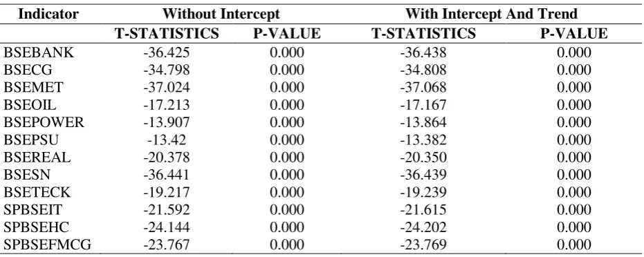
[image:11.595.75.541.541.727.2]The stationarity test for each price indices is done through Augmented Dickey – Fuller Test (ADF Test). The price indices are stationary and statically significant at 1 percent, after first.
Table 1: Descriptive Statistics
Indicator Mean Std.Dev Variance skewness Kurtosis BSESN -8.75 218.12 47578.34 0.34 5.62 BSEPSU -5.48 225.41 50811.31 -30.91 1125.21 BSEPOWER -1.42 69.33 4806.26 -31.29 1144.56 BSEOIL -8.86 267.93 71783.89 -27.77 976.91 BSEREAL -1.28 60.45 3653.92 -21.62 701.45 BSETECK -3.63 105.01 11027.38 -25.50 873.63 BSEMET 2.55 166.66 27776.61 -0.07 4.29 BSEBANK -9.76 227.69 51840.60 0.07 5.00 BSECG -3.41 189.60 35948.35 0.00 6.46 SPBSEHC -9.13 197.10 38849.73 -15.21 453.40 SPBSEFMCG -6.51 107.87 11635.53 -16.81 504.23 SPBSEIT -6.48 188.96 35705.29 -21.98 719.56
Clustering Volatility test. ARCH models
After that, we ran all ARCH models to checked the ARCH effects (i.e. conditional volatility)
for subgroups of the BSE SENSEX Indices through Z- statistics.
For test of heteroscedasticity, ARCH-LM test is used. A statistically significant coefficient
indicates the presence of ARCH effect in the residuals of mean equation of BSE SENSEX. The
ARCH-Test is a portmanteau test. It tests a number of lags (lag 1 through lag q) at once as a
group and indicates whether the average ARCH effect within the group is large. The maximum
lag q governs the trade-off between power and generality. One of the most important issues
before applying the ARCH methodology is to first examine the residuals for the evidence of
heteroscedasticity. Therefore, to test the presence of heteroscedasticity in residual of the return
series, Lagrange Multiplier (LM) test is used.
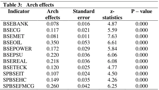
Table 3. explains about the conditional variance of the series of BSE SENSEX. We have estimated the
ARCH effects for all indices at 5% significant level. We found that in BSEOIL index, there is ARCH
effect of other indices like stocks of BSEREAL, BSETECK, SPBSEFMCG and BSECG in the BSE
market. There are various reasons behind high clustering volatility. If the returns of BSEOIL increases
or decreases its means that oil shocks have impacts on various goods and services and other indices in
the financial market because oil is a tradable commodity. Some factors are really affecting to financial
market, for example, if the exchange rate variation and any types of policies changes also affects BSE
SENSEX index.
GARCH Model
Another model we used for the forecasting is the GARCH model, which measured the unconditional
[image:12.595.136.460.494.677.2]variance of the shocks or innovations in the financial market. It has estimated the volatility of Table 3: Arch effects
Indicator Arch effects
Standard error
z- statistics
unobservable series returns. We estimated the GARCH effects for all respective indices. We found the
GARCH effect which is described in the table 4.
The null hypothesis of ‘no arch effect’ is rejected at 1% level, which estimates the presence of arch effects in the errors terms of time series models in the stocks returns and hence the results
require for the estimation of GARCH family models.
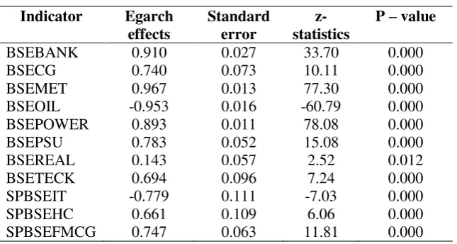
EGARCH Model
Our next model is the EGARCH model, which tells about asymmetric information’s of stock’s returns in the financial market. But it unable to capture the conditional variance of stocks. Table 5 represents
EGARCH effect is positive in BSEPOWER and BSEMET, but in BSEOIL there is negative effects.
EGARCH effect is greater in BSEPOWER (0.89) followed by BSEMET (0.96), but in the case
of BSEOIL ( -0.95) it is negative. In the BSE market get influenced because oil is a tradable
[image:13.595.138.459.186.365.2]goods and services. Its impacts will create imbalances in BSE SENSEX
Table 4: Garch effects Indicator Garch
effects
Standard error
z- statistics
P – value BSEBANK 0.819 0.042 19.52 0.000 BSECG 0.621 0.074 8.43 0.000 BSEMET 0.887 0.018 49.47 0.000 BSEOIL 0.461 0.075 6.12 0.000 BSEPOWER 0.543 0.101 5.36 0.000 BSEPSU 0.531 0.091 5.86 0.000 BSEREAL 0.510 0.093 5.46 0.000 BSETECK 0.558 0.129 4.33 0.000 SPBSEIT 0.552 0.142 3.88 0.000 SPBSEHC 0.529 0.124 4.26 0.000 SPBSEFMCG 0.543 0.086 6.30 0.000
Table 5: EGARCH Effects
Indicator Egarch effects
Standard error
z- statistics
[image:13.595.138.461.579.751.2]TGARCH Model
TGARCH and GJR TGARCH captures the “Leverage effect “of series returns. There is a relationship between the negative and positive shocks or innovations. The asymmetrical
TGARCH model which is used to estimate the returns of BSE SENSEX which is presented in
the table 6. Our analysis revealed that there is a negative correlation between past return and
future return (leverage effect). The EGARCH model supports for the presence of leverage
effect BSE SENSEX return series.
/
GJR TGARCH Model
It is also showing the same GJR TARCH effects in BSEREAL (0.98) and in BSETECK (0.67), here the positive shocks or innovations are greater than the negative shocks or returns
in the markets. The booms which is occurred in the BSE SENSEX. It is the drawbacks of
GRACH model, which has shown in our table 7.
[image:14.595.138.460.248.430.2]
Table 6: TGARCH Effects
Indicator Tgarch effects
Standard error
z- statistics
[image:14.595.137.459.568.760.2]P – value BSEBANK -0.116 0.034 -3.45 0.001 BSECG -0.129 0.031 -4.23 0.000 BSEMET -0.077 0.034 -2.24 0.025 BSEOIL 0.169 0.037 4.63 0.000 BSEPOWER 0.126 0.033 3.78 0.000 BSEPSU 0.156 0.035 4.51 0.000 BSEREAL 0.335 0.051 6.57 0.000 BSETECK 0.117 0.033 3.51 0.000 SPBSEIT 0.095 0.032 2.91 0.004 SPBSEHC 0.099 0.032 3.11 0.002 SPBSEFMCG 0.120 0.035 3.46 0.001
Table 7: GJR TARCH Effects
Indicator GJR Tarch effects Standard error z- statistics
P – value
SAARCH Model
In table 8, the negative shocks or innovations highly from BSEOIL ( -0.90) which have negative impacts on other goods and services markets. Because it is a tradable commodity from
other exportable country which affects most of the other price indices BSEPSU (- 0.90)
BSEREAL ( -0.87) SPBSEFMCG ( -0.89) and BSETECK ( -0.82) there is SAARCH effects
in the BSE markets. It is the main important cause to variation in stocks. Which shows the
relationship between asymmetric volatility and return.
PARCH Model
There are alternate models to measure asymmetric information’s like goods news and bad news of the return series. Such models are GJR TARCH, SAARCH, PARCH, these models are
actually the drawbacks of the GARCH model. PARCH model which is estimating the ARCH
effect through the power asymmetric returns series.
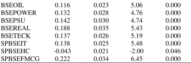
We observed from the given above Table 9, that is the POWER ARCH effect which is nothing as the “Leverage effect” through power. It follows GARCH models, the PARCH effects found in SPBSEFMCG (0.22) which positively affect to other indices, BSEBANK
[image:15.595.138.459.234.441.2](0.09) and in BSECG (0.11).
Table 8. SAARCH Effects
Indicator Simple asymmetric Arch effects
Standard error
z- statistics
P – value
BSEBANK -0.821 0.309 -2.65 0.008 BSECG -0.717 0.191 -3.75 0.000 BSEMET -0.544 0.452 -1.20 0.229 BSEOIL -0.910 0.067 -13.56 0.000 BSEPOWER -0.912 0.078 -11.70 0.000 BSEPSU -0.905 0.070 -13.01 0.000 BSEREAL -0.870 0.069 -12.68 0.000 BSETECK -0.820 0.098 -8.41 0.000 SPBSEIT -0.795 0.106 -7.50 0.000 SPBSEHC -0.748 0.117 -6.38 0.000 SPBSEFMCG -0.894 0.082 -10.91 0.000
Table 9. PARCH Effects
Indicator Parch effects
Standard error
z- statistics
P – value BSEBANK 0.092 0.016 5.78 0.000 BSECG 0.118 0.021
0.011
NARCH Model
Others models like NARCH, NARCH with one shift, APARCH and NAPARCH, these models
are measuring all those asymmetric volatility and symmetric relationship between of negative
and positive shocks or innovations in the BSE SENSEX. Our study found that implies the
negative shocks or bad news have a greater effect on the conditional volatility than the positive
shocks or good news, which shows that the variance equation is well recognised for the Indian
stock (BSE) markets. From table 10, NARCH effects found mostly in BSEOIL (0.35) and its followed by other indices as SPBSEFMCG (0.26) BSEREAL (0.22) and BSEPSU (0.22).
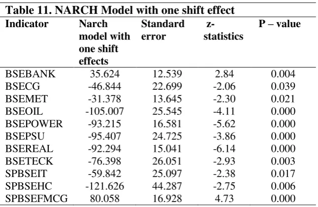
Nonlinear arch with one shift Model (NARCHK)
Nonlinear arch with one shift effects means unobservable variation, which is the asymmetric
volatility of its past one period lag shocks. Mostly we found negative arch effects in BSEREAL
( -92) BSEOIL ( -105) and positive in SPBSEFMCG (80. 05) and BSETECK (- 76.39). Which is
shown under the given table 11.
[image:16.595.141.454.70.174.2]
BSEOIL 0.116 0.023 5.06 0.000 BSEPOWER 0.132 0.028 4.76 0.000 BSEPSU 0.142 0.030 4.74 0.000 BSEREAL 0.188 0.035 5.43 0.000 BSETECK 0.137 0.026 5.19 0.000 SPBSEIT 0.138 0.025 5.48 0.000 SPBSEHC -0.043 0.021 -2.00 0.046 SPBSEFMCG 0.222 0.034 6.45 0.000
Table 10. NARCH Effects
Indicator Narch effects
Standard error
z- statistics
APARCH Model
APARCH effect shown in table 12, the positive and negative have equal magnitudes.
NPARCH Model
NPARCH effects which shows in the indices like more in BSEPSU (0.45) its followed
BSEREAL (0.30) BSETECK (0.25) and SPBSEIT (0.20). There is minimum variance which
lies between positive and negative value of shocks and innovations.
Given below table 14. We studied about the correlation between the indices and its returns
also to calculated the deviations. Our ARCH model measure the regularity of conditional
variance and our drawbacks of GARCH, EGARCH and TGARCH model which are best model
to find out the asymmetric volatility clustering. Above that shown the negative correlation
[image:17.595.137.460.53.263.2]coefficient in BSEPOWER (-0.694) and BSEPSU (-0.782). Table 11. NARCH Model with one shift effect
Indicator Narch model with one shift effects
Standard error
z- statistics
P – value
[image:17.595.135.463.344.526.2]BSEBANK 35.624 12.539 2.84 0.004 BSECG -46.844 22.699 -2.06 0.039 BSEMET -31.378 13.645 -2.30 0.021 BSEOIL -105.007 25.545 -4.11 0.000 BSEPOWER -93.215 16.581 -5.62 0.000 BSEPSU -95.407 24.725 -3.86 0.000 BSEREAL -92.294 15.041 -6.14 0.000 BSETECK -76.398 26.051 -2.93 0.003 SPBSEIT -59.842 25.097 -2.38 0.017 SPBSEHC -121.626 44.287 -2.75 0.006 SPBSEFMCG 80.058 16.928 4.73 0.000
Table 12. APARCH Effects Indicator Aparch
effects
Standard error
Conclusions
One an important objective of our paper is that to investigate volatility clustering of the BSE
SENSEX returns series through using various ARCH FAMILY models. The study is based on the secondary data sources that were collected from the data base of Bombay stock market.
(BSE) indices are used as proxy of Indian stock market. With the availability of high frequency
data being compiled by Bombay stock exchange (BSE). The data is collected on the daily prices
of BSE SENSEX indices over the period of seven years from 1st January 2011 to 1st January
2017. Our data set is the time series, which is daily data of the closing price of stock market.
GARCH, EGARCH and TGARCH models have been employed for this study after confirming
the unit root test, volatility clustering and ARCH effect. Modelling and forecasting volatility
of stock markets, it is an important field to analysis and research in financial economics time
series.
Various Conditional volatility models (ARCH/GARCH) asymmetric responded volatility to
movement of stock markets and investigate the ARCH effects. Our results show that while
conditional volatility models estimating volatility for the past series, extreme value estimators
based on trading range perform well on efficiency. This value estimators act well to forecast
the daily or our data is five-days we can say weekend effect and one month (30 days) volatility
ahead much best than the conditional volatility models.
There is an ARCH effect in BSEOIL found which is affecting all the indices in the BSE
SENSEX market. We also found in our study that the BSEREAL also have volatility clustering
in the stock markets because the price of real estate differs according its forms of land and we
can see in the case of BSEBANK and SPBSEIT both are performing as an important dominants
indicator in the BSE market.
Table 13. NPARCH Effects
Indicator Nparch effect
Standard error
z- statistics
PGARCH model results shows significant influence in terms of power on the conditional
volatility. If we see in our present era of global integration of emerging stock markets like India
with other world major stock markets, there is leverage effect which is present in the Indian
stock market indicates that negative shocks have greater impacts on the International markets
can easily external or spill over effect on our Indian stock markets, which clearly shows that it
affects adversely to the Indian stock markets and it was proved from global financial crisis in
2008. The volatility of BSE stock returns has estimated and modelled two models which is
asymmetric nonlinear models EGARCH and TGARCH and news impact curve. The results
represent that the volatility in the Indian stock market exhibits the persistence of volatility and
mean reverting behaviour. In our study we found that BSE Sensex returns series responded
leverage effects and to summed of others stylized facts such as volatility clustering and
leptokurtosis represented as a stock returns on International stock markets. Our ARCH model
measure the regularity of conditional variance and our drawbacks of GARCH, EGARCH and
TGARCH model which are best model to find out the asymmetric volatility clustering. We
studied about the correlation between the indices and its returns also to calculated the
deviations You can see the appendix, the indicators are BSEBANK, BSECG, BSEMET and
BSEOIL have positive impact on BSE SENSE and other hand the negative in BSEPOWER
(-0.694) and BSEPSU (-0.782).
Appendix
References
Ruey S. Tsay “Analysis of financial time series “A JOHN WILEY & SONS, INC., PUBLICATION
INDICATORS BSE
BANK BSE CG BSE MET BSE OIL BSE POWE R BSE PSU BSE REAL BSE TECK SPBSE IT SPBSE HC SPBSE FMCG ARCH MODEL
0.533 0.273 0.329 0.399 -0.694 -0.781 -0.224 0.590 0.117 0.085 0.553
EGARCH MODEL
0.536 0.271 0.330 0.399 -0.685 -0.782 -0.230 0.590 0.115 0.083 0.553
TARCH MODEL
0.536 0.271 0.330 0.399 -0.685 -0.782 -0.230 0.590 0.115 0.083 0.553
Standard error
Karunanithy Banumathy Kanchi Mamunivar and Ramachandran Azhagaiah Kanchi Mamuniva “Modelling Stock Market Volatility: Evidence from India “Managing Global Transitions 13 (1): 27–42
CMA Potharla Srikanth, “Modelling Stock Market Volatility: Evidence from India Modelling Asymmetric Volatility in Indian Stock Market”. Pacific Business Review International Volume 6, Issue 9, March 2014
Michael Mckenzie and Healther Mitchell “Generalised Asymmetric Power ARCH Modelling of Exchange Rate Volatility”.
Greg N. Gregarious and Razvan Pascalau “Nonlinear Financial Econometrics: Forecasting Models, Computational and Bayesian model “. Palgrave Macmillan, publication 2011.
Snehal Bandivadekar and Saurabh Ghosh “Derivatives and volatility on Indian Stock Markets “Reserve Bank of India Occasional Papers Vol. 24, No. 3 Winter 200
Madhusudan C Karmaker. “Modelling Conditional Volatility of the Stock Markets “.
VIKALPA • VOLUME 30 • NO 3 • JULY - SEPTEMBER 2005
Hojatallah Goudarzi and C.S. Ramanarayanam “Modelling Asymmetric Volatility in Indian
Stock Market “. International Journal of Business and Management.
Ramaprasad Bhar “Return and Volatility Dynamics in the Spot and Futures Markets in
Australia: An Intervention Analysis in a Bivariate EGARCH-X Framework”.Copyright © 2001 John Wiley & Sons, Inc.
Suleyman Gockan, “Forecasting Volatility of Emerging Stock Markets: Linear versus Non
-linear GARCH Models “. Journal of forecasting, volume 19, issue 6 November 2000.
Saurabh Singh and Dr. L.K Tripathi,”Modelling Stock Market Return Volatility: Evidence
from India”. Research Journal of Financial and Accounting ISSN 2222-1697 (Paper) ISSN
2222-2847 (Online) Vol.7, No.13,2016.
Ajay Pandey,” Volatility Models and their Performance in Indian Capital Markets.” VIKALPA •
VOLUME 30 • NO 2 • APRIL - JUNE 2005.
Dr. Premalata Shenbagaraman,” Do Futures and Options trading increase stock market volatility?” CFA, Department of Finance, Clemson University, Clemson, USA. The views expressed and the approach suggested are of the authors and not necessarily of NSE.
Hojatallah goudarzi,” Modelling and Estimation of Volatility in The Indian Stock Markets”. International Journal of Business and Management ISSN 1833-3850 (Print) ISSN 1833-8119 (Online).
Bollerslev, Tim. (1986). Generalized autoregressive conditional heteroscedasticity. journal of
Econometrics, Vol, 31,307-327
Tsuji Chickasha. (2003). Is volatility the best predictor of market crashes? Asia pacific