Learning to Skim Text

Proceedings of the 55th Annual Meeting of the Association for Computational Linguistics, pages 1880–1890 Vancouver, Canada, July 30 - August 4, 2017. c2017 Association for Computational Linguistics Proceedings of the 55th Annual Meeting of the Association for Computational Linguistics, pages 1880–1890

Vancouver, Canada, July 30 - August 4, 2017. c2017 Association for Computational Linguistics

Learning to Skim Text

Adams Wei Yu∗

Carnegie Mellon University [email protected]

Hongrae Lee Google

[email protected]

Quoc V. Le Google [email protected]

Abstract

Recurrent Neural Networks are showing much promise in many sub-areas of nat-ural language processing, ranging from document classification to machine trans-lation to automatic question answering. Despite their promise, many recurrent models have to read the whole text word by word, making it slow to handle long documents. For example, it is difficult to use a recurrent network to read a book and answer questions about it. In this paper, we present an approach of read-ing text while skippread-ing irrelevant informa-tion if needed. The underlying model is a recurrent network that learns how far to jump after reading a few words of the input text. We employ a standard policy gradient method to train the model to make discrete jumping decisions. In our benchmarks on four different tasks, including number prediction, sentiment analysis, news arti-cle classification and automatic Q&A, our proposed model, a modified LSTM with jumping, is up to 6 times faster than the standard sequential LSTM, while main-taining the same or even better accuracy.

1 Introduction

The last few years have seen much success of ap-plying neural networks to many important appli-cations in natural language processing, e.g., part-of-speech tagging, chunking, named entity recog-nition (Collobert et al., 2011), sentiment analy-sis (Socher et al.,2011,2013), document classifi-cation (Kim,2014;Le and Mikolov,2014;Zhang et al.,2015;Dai and Le, 2015), machine transla-tion (Kalchbrenner and Blunsom,2013;Sutskever

∗_{Most of work was done when AWY was with Google.}

et al.,2014;Bahdanau et al.,2014;Sennrich et al.,

2015; Wu et al., 2016), conversational/dialogue modeling (Sordoni et al., 2015; Vinyals and Le,

2015;Shang et al., 2015), document summariza-tion (Rush et al., 2015; Nallapati et al., 2016), parsing (Andor et al.,2016) and automatic ques-tion answering (Q&A) (Weston et al.,2015; Her-mann et al., 2015; Wang and Jiang, 2016; Wang et al.,2016;Trischler et al.,2016;Lee et al.,2016;

Seo et al.,2016;Xiong et al.,2016). An important characteristic of all these models is that they read all the text available to them. While it is essential for certain applications, such as machine transla-tion, this characteristic also makes it slow to ap-ply these models to scenarios that have long input text, such as document classification or automatic Q&A. However, the fact that texts are usually writ-ten with redundancy inspires us to think about the possibility of reading selectively.

In this paper, we consider the problem of under-standing documents with partial reading, and pro-pose a modification to the basic neural architec-tures that allows them to read input text with skip-ping. The main benefit of this approach is faster inference because it skips irrelevant information. An unexpected benefit of this approach is that it also helps the models generalize better.

In our approach, the model is a recurrent net-work, which learns to predict the number of jump-ing steps after it reads one or several input tokens. Such a discrete model is therefore not fully differ-entiable, but it can be trained by a standard policy gradient algorithm, where the reward can be the accuracy or its proxy during training.

In our experiments, we use the basic LSTM recurrent networks (Hochreiter and Schmidhuber,

1997) as the base model and benchmark the pro-posed algorithm on a range of document clas-sification or reading comprehension tasks, using various datasets such as Rotten Tomatoes (Pang

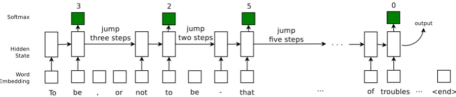
Figure 1: A synthetic example of the proposed model to process a text document. In this example, the maximum size of jumpKis 5, the number of tokens read before a jumpRis 2 and the number of jumps allowedN is 10. The green softmax are for jumping predictions. The processing stops if a) the jumping softmax predicts a 0 or b) the jump times exceedsN or c) the network processed the last token. We only show the case a) in this figure.

and Lee, 2005), IMDB (Maas et al., 2011), AG News (Zhang et al., 2015) and Children’s Book Test (Hill et al.,2015). We find that the proposed approach of selective reading speeds up the base model by two to six times. Surprisingly, we also observe our model beats the standard LSTM in terms of accuracy.

In summary, the main contribution of our work is to design an architecture that learns to skim text and show that it is both faster and more accurate in practical applications of text processing. Our model is simple and flexible enough that we antic-ipate it would be able to incorporate to recurrent nets with more sophisticated structures to achieve even better performance in the future.

2 Methodology

In this section, we introduce the proposed model named LSTM-Jump. We first describe its main structure, followed by the difficulty of estimat-ing part of the model parameters because of non-differentiability. To address this issue, we appeal to a reinforcement learning formulation and adopt a policy gradient method.

2.1 Model Overview

The main architecture of the proposed model is shown in Figure1, which is based on an LSTM re-current neural network. Before training, the num-ber of jumps allowed N, the number of tokens read between every two jumps R and the max-imum size of jumping K are chosen ahead of time. WhileK is a fixed parameter of the model, N and R are hyperparameters that can vary be-tween training and testing. Also, throughout the paper, we would use d1:p to denote a sequence d1, d2, ..., dp.

In the following, we describe in detail how the model operates when processing text. Given a training examplex1:T, the recurrent network will read the embedding of the firstRtokensx1:Rand output the hidden state. Then this state is used to compute the jumping softmax that determines a distribution over the jumping steps between1and

K. The model then samples from this distribution a jumping step, which is used to decide the next token to be read into the model. Letκbe the sam-pled value, then the next starting token isxR+κ. Such process continues until either

a) the jump softmax samples a 0; or b) the number of jumps exceedsN; or c) the model reaches the last tokenxT.

After stopping, as the output, the latest hidden state is further used for predicting desired targets. How to leverage the hidden state depends on the specifics of the task at hand. For example, for clas-sification problems in Section3.1, 3.2and3.3, it is directly applied to produce a softmax for classi-fication, while in automatic Q&A problem of Sec-tion3.4, it is used to compute the correlation with the candidate answers in order to select the best one. Figure 1 gives an example with K = 5, R= 2andN = 10terminating on condition a).

2.2 Training with REINFORCE

Our goal for training is to estimate the parameters of LSTM and possibly word embedding, which are denoted asθm, together with the jumping ac-tion parameters θa. Once obtained, they can be used for inference.

differentiable overθm that we can directly apply backpropagation to minimize.

However, the nature of discrete jumping deci-sions made at every step makes it difficult to es-timateθa, as cross entropy is no longer differen-tiable over θa. Therefore, we formulate it as a reinforcement learning problem and apply policy gradient method to train the model. Specifically, we need to maximize a reward function over θa which can be constructed as follows.

Let j1:N be the jumping action sequence dur-ing the traindur-ing with an example x1:T. Suppose hi is a hidden state of the LSTM right before the i-th jump ji,1 then it is a function of j1:i−1 and

thus can be denoted ashi(j1:i−1). Now the jump

is attained by sampling from the multinomial dis-tributionp(ji|hi(j1:i−1);θa), which is determined

by the jump softmax. We can receive a reward Rafter processingx1:T under the current jumping strategy.2_{The reward should be positive if the} out-put is favorable or non-positive otherwise. In our experiments, we choose

R=

1 if prediction correct; −1 otherwise.

Then the objective function ofθawe want to max-imize is the expected reward under the distribution defined by the current jumping policy, i.e.,

J2(θa) =Ep(j1:N;θa)[R]. (1)

wherep(j1:N;θa) =Q_ip(j1:i|hi(j1:i−1);θa). Optimizing this objective numerically requires computing its gradient, whose exact value is in-tractable to obtain as the expectation is over high dimensional interaction sequences. By running S examples, an approximated gradient can be computed by the following REINFORCE algo-rithm (Williams,1992):

∇θaJ2(θa) =

N

X

i=1

Ep(j1:N;θa)[∇θalogp(j1:i|hi;θa)R]

≈1

S S

X

s=1

N

X

i=1

[∇θalogp(j

s

1:i|hsi;θa)Rs]

where the superscript s denotes a quantity be-longing to the s-th example. Now the term

1_{Thei-th jumping step is usuallynotxi.}

2_{In the general case, one may receive (discounted)} inter-mediate rewards after each jump. But in our case, we only consider final reward. It is equivalent to a special case that all intermediate rewards are identical and without discount.

∇θalogp(j1:i|hi;θa) can be computed by

stan-dard backpropagation.

Although the above estimation of∇θaJ2(θa)is

unbiased, it may have very high variance. One widely used remedy to reduce the variance is to subtract abaselinevalue bs

i from the reward Rs, such that the approximated gradient becomes

∇θaJ2(θa)≈

1

S S

X

s=1

N

X

i=1

[∇θalogp(j

s

1:i|hsi;θ)(Rs−bsi)]

It is shown (Williams, 1992; Zaremba and Sutskever,2015) that any numberbs_i will yield an unbiased estimation. Here, we adopt the strategy ofMnih et al.(2014) thatbs

i =wbhsi +cband the parameterθb ={wb, cb}is learned by minimizing

(Rs₋bs_i)2. Now the final objective to minimize is

J(θm, θa, θb) =J1(θm)−J2(θa)+ S

X

s=1

N

X

i=1

(Rs₋bs_i)2,

which is fully differentiable and can be solved by standard backpropagation.

2.3 Inference

During inference, we can either use sampling or greedy evaluation by selecting the most probable jumping step suggested by the jump softmax and follow that path. In the our experiments, we will adopt the sampling scheme.

3 Experimental Results

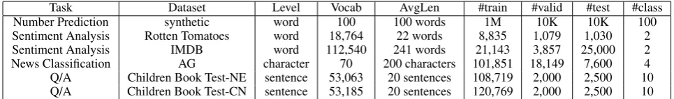
In this section, we present our empirical studies to understand the efficiency of the proposed model in reading text. The tasks under experimentation are: synthetic number prediction, sentiment analysis, news topic classification and automatic question answering. Those, except the first one, are repre-sentative tasks in text reading involving different sizes of datasets and various levels of text process-ing, from character to word and to sentence. Ta-ble1summarizes the statistics of the dataset in our experiments.

To exclude the potential impact of advanced models, we restrict our comparison between the vanilla LSTM (Hochreiter and Schmidhuber,

Task Dataset Level Vocab AvgLen #train #valid #test #class

Number Prediction synthetic word 100 100 words 1M 10K 10K 100

Sentiment Analysis Rotten Tomatoes word 18,764 22 words 8,835 1,079 1,030 2 Sentiment Analysis IMDB word 112,540 241 words 21,143 3,857 25,000 2 News Classification AG character 70 200 characters 101,851 18,149 7,600 4 Q/A Children Book Test-NE sentence 53,063 20 sentences 108,719 2,000 2,500 10 Q/A Children Book Test-CN sentence 53,185 20 sentences 120,769 2,000 2,500 10

Table 1: Task and dataset statistics.

datasets, respectively, as we are able to selectively skip a large fraction of text.

In fact, the proposed model can be readily ex-tended to other recurrent neural networks with so-phisticated mechanisms such as attention and/or hierarchical structure to achieve higher accuracy than those presented below. However, this is or-thogonal to the main focus of this work and would be left as an interesting future work.

General Experiment Settings We use the Adam optimizer (Kingma and Ba, 2014) with a learning rate of 0.001 in all experiments. We also apply gradient clipping to all the trainable vari-ables with the threshold of 1.0. The dropout rate between the LSTM layers is 0.2 and the embed-ding dropout rate is 0.1. We repeat the notations N, K, Rdefined previously in Table2, so readers can easily refer to when looking at Tables 4,5,6

and7. WhileK is fixed during both training and testing, we would fixRandN at training but vary their values during test to see the impact of pa-rameter changes. Note thatN is essentially a con-straint which can be relaxed. Yet we prefer to en-force this constraint here to let the model learn to read fewer tokens. Finally, the reported test time is measured by running one pass of the whole test set instance by instance, and the speedup is over the base LSTM model. The code is written with TensorFlow.3

Notation Meaning

N number of jumps allowed

K maximum size of jumping

R number of tokens read before a jump

Table 2: Notations referred to in experiments.

3.1 Number Prediction with a Synthetic Dataset

We first test whether LSTM-Jump is indeed able to learn how to jump if avery clearjumping

sig-3_{https://www.tensorflow.org/}

nal is given in the text. The input of the task is a sequence ofL positive integersx0:T−1 and the

output is simplyxx0. That is, the output is chosen from the input sequence, with index determined by x0. Here are two examples to illustrate the idea:

input1: 4,5,1,7,6,2. output1: 6

input2: 2,4,9,4,5,6. output2: 9

One can see thatx0is essentially the oracle

jump-ing signal, i.e. the indicator of how many steps the reading should jump to get the exact output and obviously, the remaining number of the sequence are useless. After reading the first token, a “smart” network should be able to learn from the training examples to jump to the output position, skipping the rest.

We generate 1 million training and 10,000 val-idation examples with the rule above, each with sequence length T = 100. We also impose 1 ≤ x0 < T to ensure the index is valid. We

find that directly training the LSTM-Jump with full sequence is unlikely to converge, therefore, we adopt a curriculum training scheme. More specifically, we generate sequences with lengths

{10,20,30,40,50,60,70,80,90,100_} and train

the model starting from the shortest. Whenever the training accuracy reaches a threshold, we shift to longer sequences. We also train an LSTM with the same curriculum training scheme. The train-ing stops when the validation accuracy is larger than98%. We choose such stopping criterion

sim-ply because it is the highest that both models can achieve.4 _{All the networks are single layered, with} hidden size 512, embedding size 32 and batch size 100. During testing, we generate sequences of lengths 10, 100 and 1000 with the same rule, each having 10,000 examples. As the training size is large enough, we do not have to worry about over-fitting so dropout is not applied. In fact, we find that the training, validation and testing accuracies are almost the same.

Seq length LSTM-Jump LSTM Speedup Test accuracy

10 98% 96% n/a

100 98% 96% n/a

1000 90% 80% n/a

Test time (Avg tokens read)

10 13.5s (2.1) 18.9s (10) 1.40x

100 13.9s (2.2) 120.4s (100) 8.66x

1000 18.9s (3.0) 1250s (1000) 66.14x

Table 3: Testing accuracy and time of synthetic number prediction problem. The jumping level is number.

The results of LSTM and our method, LSTM-Jump, are shown in Table 3. The first observa-tion is that LSTM-Jump is faster than LSTM; the longer the sequence is, the more significant speed-up LSTM-Jump can gain. This is because the well-trained LSTM-Jump is aware of the jump-ing signal at the first token and hence can directly jump to the output position to make prediction, while LSTM is agnostic to the signal and has to read the whole sequence. As a result, the read-ing speed of LSTM-Jump is hardly affected by the length of sequence, but that of LSTM is linear with respect to length. Besides, LSTM-Jump also out-performs LSTM in terms of test accuracy under all cases. This is not surprising either, as LSTM has to read a large amount of tokens that are potentially not helpful and could interfere with the prediction. In summary, the results indicate LSTM-Jump is able to learn to jump if the signal is clear.

3.2 Word Level Sentiment Analysis with Rotten Tomatoes and IMDB datasets As LSTM-Jump has shown great speedups in the synthetic dataset, we would like to understand whether it could carry this benefit to real-world data, where “jumping” signal is not explicit. So in this section, we conduct sentiment analysis on two movie review datasets, both containing equal numbers of positive and negative reviews.

The first dataset is Rotten Tomatoes, which con-tains 10,662 documents. Since there is not a stan-dard split, we randomly select around 80% for training, 10% for validation, and 10% for test-ing. The average and maximum lengths of the re-views are 22 and 56 words respectively, and we pad each of them to 60. We choose the pre-trained word2vec embeddings5 _{(Mikolov et al.,2013) as}

5_{https://code.google.com/archive/p/} word2vec/

our fixed word embedding that we do not update this matrix during training. Both LSTM-Jump and LSTM contain 2 layers, 256 hidden units and the batch size is 100. As the amount of training data is small, we slightly augment the data by sampling a continuous 50-word sequence in each padded re-views as one training sample. During training, we enforce LSTM-Jump to read 8 tokens before a jump (R = 8), and the maximum skipping

to-kens per jump is 10 (K = 10), while the number

of jumps allowed is 3 (N = 3).

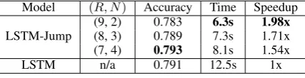
The testing result is reported in Table 4. In a nutshell, LSTM-Jump is always faster than LSTM under different combinations ofRandN. At the same time, the accuracy is on par with that of LSTM. In particular, the combination of(R, N) = (7,4)even achieves slightly better accuracy than

LSTM while having a 1.5x speedup.

Model (R, N) Accuracy Time Speedup LSTM-Jump (9, 2)(8, 3) 0.7830.789 6.3s7.3s 1.98x1.71x

(7, 4) 0.793 8.1s 1.54x

LSTM n/a 0.791 12.5s 1x

Table 4: Testing time and accuracy on the Rotten Tomatoes review classification dataset. The max-imum size of jumping K is set to 10 for all the

settings. The jumping level is word.

The second dataset is IMDB (Maas et al.,

2011),6_{which contains 25,000 training and 25,000} testing movie reviews, where the average length of text is 240 words, much longer than that of Rotten Tomatoes. We randomly set aside about 15% of training data as validation set. Both LSTM-Jump and LSTM has one layer and 128 hidden units, and the batch size is 50. Again, we use pretrained word2vec embeddings as initialization but they are updated during training. We either pad a short se-quence to 400 words or randomly select a 400-word segment from a long sequence as a training example. During training, we setR= 20, K = 40

andN = 5.

As Table5 shows, the result exhibits a similar trend as found in Rotten Tomatoes that LSTM-Jump is uniformly faster than LSTM under many settings. The various(R, N) combinations again demonstrate the trade-off between efficiency and accuracy. If one cares more about accuracy, then allowing LSTM-Jump to read and jump more

Model (R, N) Accuracy Time Speedup

LSTM-Jump

(80, 8) 0.894 769s 1.62x (80, 3) 0.892 764s 1.63x (70, 3) 0.889 673s 1.85x (50, 2) 0.887 585s 2.12x (100, 1) 0.880 489s 2.54x

LSTM n/a 0.891 1243s 1x

Table 5: Testing time and accuracy on the IMDB sentiment analysis dataset. The maximum size of jumping K is set to40 for all the settings. The

jumping level is word.

times is a good choice. Otherwise, shrinking ei-ther one would bring a significant speedup though at the price of losing some accuracy. Neverthe-less, the configuration with the highest accuracy still enjoys a 1.6x speedup compared to LSTM. With a slight loss of accuracy, LSTM-Jump can be 2.5x faster .

3.3 Character Level News Article Classification with AG dataset

We now present results on testing the character level jumping with a news article classification problem. The dataset contains four classes of top-ics (World, Sports, Business, Sci/Tech) from the AG’s news corpus,7 _{a collection of more than 1} million news articles. The data we use is the subset constructed by Zhang et al.(2015) for classifica-tion with character-level convoluclassifica-tional networks. There are 30,000 training and 1,900 testing ex-amples for each class respectively, where 15% of training data is set aside as validation. The non-space alphabet under use are:

abcdefghijklmnopqrstuvwxyz0123456 789-,;.!?:/\|_@#$%&*˜‘+-=<>()[]{}

Since the vocabulary size is small, we choose 16 as the embedding size. The initialized entries of the embedding matrix are drawn from a uniform dis-tribution in[−0.25,0.25], which are progressively

updated during training. Both LSTM-Jump and LSTM have 1 layer and 64 hidden units and the batch sizes are 20 and 100 respectively. The train-ing sequence is again of length 400 that it is either padded from a short sequence or sampled from a long one. During training, we setR= 30, K = 40

andN = 5.

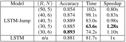
The result is summarized in Table6. It is inter-esting to see that even with skipping, LSTM-Jump

7_{http://www.di.unipi.it/˜gulli/AG_} corpus_of_news_articles.html

is not always faster than LSTM. This is mainly due to the fact that the embedding size and hidden layer are both much smaller than those used previ-ously, and accordingly the processing of a token is much faster. In that case, other computation over-head such as calculating and sampling from the jump softmax might become a dominating factor of efficiency. By this cross-task comparison, we can see that the larger the hidden unit size of re-current neural network and the embedding are, the more speedup LSTM-Jump can gain, which is also confirmed by the task below.

Model (R, N) Accuracy Time Speedup

LSTM-Jump

(50, 5) 0.854 102s 0.80x (40, 6) 0.874 98.1s 0.83x (40, 5) 0.889 83.0s 0.98x (30, 5) 0.885 63.6s 1.28x

(30, 6) 0.893 74.2s 1.10x

LSTM n/a 0.881 81.7s 1x

Table 6: Testing time and accuracy on the AG news classification dataset. The maximum size of jumpingK is set to40 for all the settings. The

jumping level is character.

3.4 Sentence Level Automatic Question Answering with Children’s Book Test dataset

The last task is automatic question answering, in which we aim to test the sentence level skimming of LSTM-Jump. We benchmark on the data set Children’s Book Test (CBT) (Hill et al., 2015).8 In each document, there are 20 contiguous sen-tences (context) extracted from a children’s book followed by a query sentence. A word of the query is deleted and the task is to select the best fit for this position from 10 candidates. Originally, there are four types of tasks according to the part of speech of the missing word, from which, we choose the most difficult two, i.e., the name en-tity (NE) and common noun (CN) as our focus, since simple language models can already achieve human-level performance for the other two types . The models, LSTM or LSTM-Jump, firstly read the whole query, then the context sentences and finally output the predicted word. While LSTM reads everything, our jumping model would de-cide how many context sentences should skip after reading one sentence. Whenever a model finishes reading, the context and query are encoded in its

hidden stateh_{o, and the best answer from the} can-didate words has the same index that maximizes the following:

softmax(CW h_o)_∈R10,

whereC ∈ R10×d _{is the word embedding matrix} of the 10 candidates andW ∈ Rd×hidden size is

a trainable weight variable. Using such bilinear form to select answer basically follows the idea ofChen et al.(2016), as it is shown to have good performance. The task is now distilled to a classi-fication problem of 10 classes.

We either truncate or pad each context sentence, such that they all have length 20. The same pre-processing is applied to the query sentences ex-cept that the length is set as 30. For both models, the number of layers is 2, the number of hidden units is 256 and the batch size is 32. Pretrained word2vec embeddings are again used and they are not adjusted during training. The maximum num-ber of context sentences LSTM-Jump can skip per time isK = 5while the number of total jumping

is limited toN = 5. We let the model jump after

reading every sentence, soR= 1(20 words). The result is reported in Table 7. The perfor-mance of LSTM-Jump is superior to LSTM in terms of both accuracy and efficiency under all set-tings in our experiments. In particular, the fastest LSTM-Jump configuration achieves a remarkable 6x speedup over LSTM, while also having respec-tively 1.4% and 4.4% higher accuracy in Chil-dren’s Book Test - Named Entity and ChilChil-dren’s Book Test - Common Noun.

Model (R, N) Accuracy Time Speedup

Children’s Book Test - Named Entity LSTM-Jump (1, 5)(1, 3) 0.4680.464 40.9s30.3s 3.04x4.11x

(1, 1) 0.452 19.9s 6.26x

LSTM n/a 0.438 124.5s 1x

Children’s Book Test - Common Noun LSTM-Jump (1, 5)(1, 3) 0.4930.487 39.3s29.7s 3.09x4.09x

(1, 1) 0.497 19.8s 6.14x

LSTM n/a 0.453 121.5s 1x

Table 7: Testing time and accuracy on the Chil-dren’s Book Test dataset. The maximum size of jumping K is set to 5 for all the settings. The

jumping level is sentence.

The dominant performance of LSTM-Jump over LSTM might be interpreted as follows. After reading the query, both LSTM and LSTM-Jump

know what the question is. However, LSTM still has to process the remaining 20 sentences and thus at the very end of the last sentence, the long de-pendency between the question and output might become weak that the prediction is hampered. On the contrary, the question can guide LSTM-Jump on how to read selectively and stop early when the answer is clear. Therefore, when it comes to the output stage, the “memory” is both fresh and un-cluttered that a more accurate answer is likely to be picked.

In the following, we show two examples of how the model reads the context given a query (bold face sentences are those read by our model in the increasing order). XXXXX is the missing word we want to fill. Note that due to truncation, a few sentences might look uncompleted.

Example 1 In the first example, the exact an-swer appears in the context multiple times, which makes the task relatively easy, as long as the reader has captured their occurrences.

(a) Query:‘XXXXX! (b) Context:

1. said Big Klaus, and he ran off at once to Little Klaus.

2. ‘Where did you get so much money from?’ 3. ‘Oh, that was from my horse-skin. 4. I sold it yesterday evening.’

5. ‘That ’s certainly a good price!’

6. said Big Klaus; and running home in great haste, he took an axe, knocked all his four 7. ‘Skins!

8. skins!

9. Who will buy skins?’ 10. he cried through the streets.

11. All the shoemakers and tanners came running to ask him what he wanted for them.’

12. A bushel of money for each,’ said Big Klaus.

13. ‘Are you mad?’ 14. they all exclaimed.

15. ‘Do you think we have money by the bushel?’ 16. ‘Skins!

17. skins!

18. Who will buy skins?’

19. he cried again, and to all who asked him what they cost, he answered,’ A bushel

20. ‘He is making game of us,’ they said; and the shoemakers seized their yard measures and (c) Candidates: Klaus | Skins | game | haste |

(d) Answer:Skins

The reading behavior might be interpreted as follows. The model tries to search for clues, and after reading sentence 8, it realizes that the most plausible answer is “Klaus” or “Skins”, as they both appear twice. “Skins” is more likely to be the answer as it is followed by a “!”. The model searches further to see if ”Klaus!” is mentioned somewhere, but it only finds “Klaus” without “!” for the third time. After the last attempt at sen-tence 14, it is confident about the answer and stops to output with “Skins”.

Example 2 In this example, the answer is illus-trated by a word “nuisance” that does not show up in the context at all. Hence, to answer the query, the model has to understand the meaning of both the query and context and locate the synonym of “nuisance”, which is not merely verbatim and thus much harder than the previous example. Neverthe-less, our model is still able to make a right choice while reading much fewer sentences.

(a) Query:Yes, I call XXXXX a nuisance. (b) Context:

1. But to you and me it would have looked just as it did to Cousin Myra – a very dis-contented

2. “I’m awfully glad to see you, Cousin Myra, ”explained Frank carefully, “and your 3. But Christmas is just a bore – a regular

bore.”

4. That was what Uncle Edgar called things that didn’t interest him, so that Frank felt pretty sure of

5. Nevertheless, he wondered uncomfortably what made Cousin Myra smile so queerly. 6. “Why, how dreadful!”

7. she said brightly.

8. “I thought all boys and girls looked upon Christmas as the very best time in the year.” 9. “We don’t, ”said Frank gloomily.

10. “It’s just the same old thing year in and year out.

11. We know just exactly what is going to hap-pen.

12. We even know pretty well what presents we are going to get.

13. And Christmas Day itself is always the same. 14. We’ll get up in the morning , and our

stock-ings will be full of thstock-ings, and half of 15. Then there ’s dinner.

16. It ’s always so poky.

17. And all the uncles and aunts come to dinner – just the same old crowd, every year, and 18. Aunt Desda always says, ‘Why, Frankie, how

you have grown!’

19. She knows I hate to be called Frankie. 20. And after dinner they’ll sit round and talk the

rest of the day, and that’s all.

(c) Candidates:Christmas|boys|day|dinner|

half|interest|rest|stockings|things|

un-cles

(d) Answer:Christmas

The reading behavior can be interpreted as fol-lows. After reading the query, our model realizes that the answer should be something like a nui-sance. Then it starts to process the text. Once it hits sentence 3, it may begin to consider “Christ-mas” as the answer, since “bore” is a synonym of “nuisance”. Yet the model is not 100% sure, so it continues to read, very conservatively – it does not jump for the next three sentences. Af-ter that, the model gains more confidence on the answer “Christmas” and it makes a large jump to see if there is something that can turn over the cur-rent hypothesis. It turns out that the last-read sen-tence is still talking about Christmas with a neg-ative voice. Therefore, the model stops to take “Christmas” as the output.

4 Related Work

Closely related to our work is the idea of learn-ing visual attention with neural networks (Mnih et al.,2014;Ba et al.,2014;Sermanet et al.,2014), where a recurrent model is used to combine vi-sual evidence at multiple fixations processed by a convolutional neural network. Similar to our ap-proach, the model is trained end-to-end using the REINFORCE algorithm (Williams,1992). How-ever, a major difference between those work and ours is that we have to sample from discrete jump-ing distribution, while they can sample from con-tinuous distribution such as Gaussian. The differ-ence is mainly due to the inborn characteristics of text and image. In fact, as pointed out by Mnih et al.(2014), it was difficult to learn policies over more than 25 possible discrete locations.

learning (Shen et al., 2016). The key difference between our work and Shen et al.(2016) is that they focus on early stopping after multiple pass of data to ensure accuracy whereas our method fo-cuses on selective reading with single pass to en-able fast processing.

The concept of “hard” attention has also been used successfully in the context of making neu-ral network predictions more interpretable (Lei et al.,2016). The key difference between our work andLei et al.(2016)’s method is that our method optimizes for faster inference, and is more dy-namic in its jumping. Likewise is the difference between our approach and the “soft” attention ap-proach by (Bahdanau et al.,2014).

Our method belongs to adaptive computation of neural networks, whose idea is recently explored by (Graves,2016;Jernite et al.,2016), where dif-ferent amount of computations are allocated dy-namically per time step. The main difference between our method and Graves; Jernite et al.’s methods is that our method can set the amount of computation to be exactly zero for many steps, thereby achieving faster scanning over texts. Even though our method requires policy gradient meth-ods to train, which is a disadvantage compared to (Graves, 2016;Jernite et al., 2016), we do not find training with policy gradient methods prob-lematic in our experiments.

At the high-level, our model can be viewed as a simplified trainable Turing machine, where the controller can move on the input tape. It is there-fore related to the prior work on Neural Turing Machines (Graves et al.,2014) and especially its RL version (Zaremba and Sutskever,2015). Com-pared to (Zaremba and Sutskever,2015), the out-put tape in our method is more simple and reward signals in our problems are less sparse, which ex-plains why our model is easy to train. It is worth noting that Zaremba and Sutskever report diffi-culty in using policy gradients to train their model. Our method, by skipping irrelevant content, shortens the length of recurrent networks, thereby addressing the vanishing or exploding gradients in them (Hochreiter et al., 2001). The baseline method itself, Long Short Term Memory ( Hochre-iter and Schmidhuber,1997), belongs to the same category of methods. In this category, there are several recent methods that try to achieve the same goal, such as having recurrent networks that oper-ate in different frequency (Koutnik et al.,2014) or

is organized in a hierarchical fashion (Chan et al.,

2015;Chung et al.,2016).

Lastly, we should point out that we are among the recent efforts that deploy reinforcement learn-ing to the field of natural language processlearn-ing, some of which have achieved encouraging re-sults in the realm of such as neural symbolic machine (Liang et al., 2017), machine reason-ing (Shen et al., 2016) and sequence genera-tion (Ranzato et al.,2015).

5 Conclusions

In this paper, we focus on learning how to skim text for fast reading. In particular, we pro-pose a “jumping” model that after reading every few tokens, it decides how many tokens should be skipped by sampling from a softmax. Such jumping behavior is modeled as a discrete de-cision making process, which can be trained by reinforcement learning algorithm such as REIN-FORCE. In four different tasks with six datasets (one synthetic and five real), we test the efficiency of the proposed method on various levels of text jumping, from character to word and then to sen-tence. The results indicate our model is several times faster than, while the accuracy is on par with the baseline LSTM model.

Acknowledgments

The authors would like to thank the Google Brain Team, especially Zhifeng Chen and Yuan Yu for helpful discussion about the implementation of this model on Tensorflow. The first author also wants to thank Chen Liang, Hanxiao Liu, Yingtao Tian, Fish Tung, Chiyuan Zhang and Yu Zhang for their help during the project. Finally, the authors appreciate the invaluable feedback from anony-mous reviewers.

References

Daniel Andor, Chris Alberti, David Weiss, Aliaksei Severyn, Alessandro Presta, Kuzman Ganchev, Slav Petrov, and Michael Collins. 2016. Globally nor-malized transition-based neural networks. arXiv preprint arXiv:1603.06042.

Jimmy Ba, Volodymyr Mnih, and Koray Kavukcuoglu. 2014. Multiple object recognition with visual atten-tion. arXiv preprint arXiv:1412.7755.

learning to align and translate. arXiv preprint arXiv:1409.0473.

William Chan, Navdeep Jaitly, Quoc V Le, and Oriol Vinyals. 2015. Listen, attend and spell. arXiv preprint arXiv:1508.01211.

Danqi Chen, Jason Bolton, and Christopher D. Man-ning. 2016. A thorough examination of the cnn/daily mail reading comprehension task. In Pro-ceedings of the 54th Annual Meeting of the Associ-ation for ComputAssoci-ational Linguistics, ACL 2016, Au-gust 7-12, 2016, Berlin, Germany, Volume 1: Long Papers.

Eunsol Choi, Daniel Hewlett, Alexandre Lacoste, Illia Polosukhin, Jakob Uszkoreit, and Jonathan Berant. 2016. Hierarchical question answering for long doc-uments. arXiv preprint arXiv:1611.01839.

Junyoung Chung, Sungjin Ahn, and Yoshua Bengio. 2016. Hierarchical multiscale recurrent neural net-works. arXiv preprint arXiv:1609.01704.

Ronan Collobert, Jason Weston, L´eon Bottou, Michael Karlen, Koray Kavukcuoglu, and Pavel Kuksa. 2011. Natural language processing (almost) from scratch. Journal of Machine Learning Research

12(Aug):2493–2537.

Andrew M. Dai and Quoc V. Le. 2015. Semi-supervised sequence learning. InAdvances in Neu-ral Information Processing Systems. pages 3079– 3087.

Alex Graves. 2016. Adaptive computation time for recurrent neural networks. arXiv preprint arXiv:1603.08983.

Alex Graves, Greg Wayne, and Ivo Danihelka. 2014. Neural turing machines. arXiv preprint arXiv:1410.5401.

Karl Moritz Hermann, Tomas Kocisky, Edward Grefenstette, Lasse Espeholt, Will Kay, Mustafa Su-leyman, and Phil Blunsom. 2015. Teaching ma-chines to read and comprehend. InAdvances in Neu-ral Information Processing Systems. pages 1693– 1701.

Felix Hill, Antoine Bordes, Sumit Chopra, and Jason Weston. 2015. The goldilocks principle: Reading children’s books with explicit memory representa-tions. arXiv:1511.02301.

Sepp Hochreiter, Yoshua Bengio, Paolo Frasconi, and J¨urgen Schmidhuber. 2001. Gradient flow in recur-rent nets: the difficulty of learning long-term depen-dencies. In S. C. Kremer and J. F. Kolen, editors,

A Field Guide to Dynamical Recurrent Neural Net-works, IEEE press.

Sepp Hochreiter and J¨urgen Schmidhuber. 1997. Long short-term memory. Neural computation

9(8):1735–1780.

Yacine Jernite, Edouard Grave, Armand Joulin, and Tomas Mikolov. 2016. Variable computation in recurrent neural networks. arXiv preprint arXiv:1611.06188.

Nal Kalchbrenner and Phil Blunsom. 2013. Recurrent continuous translation models. InEMNLP.

Yoon Kim. 2014. Convolutional neural net-works for sentence classification. arXiv preprint arXiv:1408.5882.

Diederik Kingma and Jimmy Ba. 2014. Adam: A method for stochastic optimization. arXiv preprint arXiv:1412.6980.

Jan Koutnik, Klaus Greff, Faustino Gomez, and Juer-gen Schmidhuber. 2014. A clockwork rnn. In Inter-national Conference on Machine Learning.

Quoc V. Le and Tomas Mikolov. 2014. Distributed rep-resentations of sentences and documents. In Inter-national Conference on Machine Learning (ICML).

Kenton Lee, Tom Kwiatkowski, Ankur Parikh, and Di-panjan Das. 2016. Learning recurrent span repre-sentations for extractive question answering. arXiv preprint arXiv:1611.01436.

Tao Lei, Regina Barzilay, and Tommi Jaakkola. 2016. Rationalizing neural predictions. arXiv preprint arXiv:1606.04155.

Chen Liang, Jonathan Berant, Quoc Le, Kenneth D. Forbus, and Ni Lao. 2017. Neural symbolic ma-chines: Learning semantic parsers on freebase with weak supervision. In Proceedings of the 55th An-nual Meeting of the Association for Computational Linguistics, ACL 2017: Long Papers.

Andrew L Maas, Raymond E Daly, Peter T. Pham, Dan Huang, Andrew Y. Ng, and Christopher Potts. 2011. Learning word vectors for sentiment analysis. In

Proceedings of the 49th Annual Meeting of the Asso-ciation for Computational Linguistics: Human Lan-guage Technologies-Volume 1. Association for Com-putational Linguistics, pages 142–150.

Tomas Mikolov, Ilya Sutskever, Kai Chen, Greg S Cor-rado, and Jeff Dean. 2013. Distributed representa-tions of words and phrases and their compositional-ity. InAdvances in neural information processing systems. pages 3111–3119.

Volodymyr Mnih, Nicolas Heess, Alex Graves, et al. 2014. Recurrent models of visual attention. In

Advances in neural information processing systems. pages 2204–2212.

Bo Pang and Lillian Lee. 2005. Seeing stars: Ex-ploiting class relationships for sentiment categoriza-tion with respect to rating scales. InProceedings of the 43rd annual meeting on association for compu-tational linguistics. Association for Computational Linguistics, pages 115–124.

Marc’Aurelio Ranzato, Sumit Chopra, Michael Auli, and Wojciech Zaremba. 2015. Sequence level training with recurrent neural networks. CoRR

abs/1511.06732. http://arxiv.org/abs/1511.06732.

Alexander M Rush, Sumit Chopra, and Jason Weston. 2015. A neural attention model for abstractive sen-tence summarization. InEmpirical Methods in Nat-ural Language Processing (EMNLP).

Rico Sennrich, Barry Haddow, and Alexandra Birch. 2015. Neural machine translation of rare words with subword units. InAnnual Meeting of the Association for Computational Linguistics (ACL).

Minjoon Seo, Aniruddha Kembhavi, Ali Farhadi, and Hannaneh Hajishirzi. 2016. Bidirectional attention flow for machine comprehension. arXiv preprint arXiv:1611.01603.

Pierre Sermanet, Andrea Frome, and Esteban Real. 2014. Attention for fine-grained categorization.

arXiv preprint arXiv:1412.7054.

Lifeng Shang, Zhengdong Lu, and Hang Li. 2015. Neural responding machine for short-text conversa-tion. InAnnual Meeting of the Association for Com-putational Linguistics (ACL).

Yelong Shen, Po-Sen Huang, Jianfeng Gao, and Weizhu Chen. 2016. Reasonet: Learning to stop reading in machine comprehension. arXiv preprint arXiv:1609.05284.

Richard Socher, Jeffrey Pennington, Eric H. Huang, Andrew Y. Ng, and Christopher D. Manning. 2011. Semi-supervised recursive autoencoders for predict-ing sentiment distributions. In Proceedings of the conference on empirical methods in natural lan-guage processing.

Richard Socher, Alex Perelygin, Jean Y. Wu, Jason Chuang, Christopher D. Manning, Andrew Y. Ng, Christopher Potts, et al. 2013. Recursive deep mod-els for semantic compositionality over a sentiment treebank. InEMNLP.

Alessandro Sordoni, Michel Galley, Michael Auli, Chris Brockett, Yangfeng Ji, Margaret Mitchell, Jian-Yun Nie, Jianfeng Gao, and Bill Dolan. 2015. A neural network approach to context-sensitive gen-eration of conversational responses. arXiv preprint arXiv:1506.06714.

Ilya Sutskever, Oriol Vinyals, and Quoc V. Le. 2014. Sequence to sequence learning with neural net-works. InAdvances in neural information process-ing systems. pages 3104–3112.

Adam Trischler, Zheng Ye, Xingdi Yuan, Jing He, Phillip Bachman, and Kaheer Suleman. 2016. A parallel-hierarchical model for machine com-prehension on sparse data. arXiv preprint arXiv:1603.08884.

Oriol Vinyals and Quoc Le. 2015. A neural conversa-tional model. arXiv preprint arXiv:1506.05869.

Shuohang Wang and Jing Jiang. 2016. Machine com-prehension using match-lstm and answer pointer.

arXiv preprint arXiv:1608.07905.

Zhiguo Wang, Haitao Mi, Wael Hamza, and Radu Florian. 2016. Multi-perspective context match-ing for machine comprehension. arXiv preprint arXiv:1612.04211.

Jason Weston, Antoine Bordes, Sumit Chopra, Alexan-der M Rush, Bart van Merri¨enboer, Armand Joulin, and Tomas Mikolov. 2015. Towards ai-complete question answering: A set of prerequisite toy tasks.

arXiv preprint arXiv:1502.05698.

Ronald J. Williams. 1992. Simple statistical gradient-following algorithms for connectionist reinforce-ment learning. Machine Learning8:229–256.

Yonghui Wu, Mike Schuster, Zhifeng Chen, Quoc V. Le, Mohammad Norouzi, Wolfgang Macherey, Maxim Krikun, Yuan Cao, Qin Gao, Klaus Macherey, et al. 2016. Google’s neural ma-chine translation system: Bridging the gap between human and machine translation. arXiv preprint arXiv:1609.08144.

Caiming Xiong, Victor Zhong, and Richard Socher. 2016. Dynamic coattention networks for question answering. arXiv preprint arXiv:1611.01604. Wojciech Zaremba and Ilya Sutskever. 2015.

Rein-forcement learning neural turing machines-revised.

arXiv preprint arXiv:1505.00521.