Calculus of variations and its application to division of forest land

JOURNAL OF FOREST SCIENCE, 50, 2004 (9): 439–446

Basic source materials for the forest evaluation are both data of the forest management plan and data of the cadas-tral documentation. The basis for correct determination of the evaluated land and stand value is its truly defined area. For the calculation of the lot and parts acreage the change-affected lots are always considered. The sum of their areas is an invariable to which the calculation of the new state should be adjusted if the admissible limit is not exceeded. The simple methods of adjustment used until now cannot be employed in more complicated cases, otherwise they do not grant the unique solution.

When we want to look for an optimum variant from the given possibilities, we have to solve the problem of

finding themaximum or minimum, i.e. the highest and the

lowest values of the studied quantities. These two terms

are embraced in the term extreme (Lat. extremum). That

is why the problems of finding the maximum or minimum are called the extremal problems. Solutions of a certain class of these problems based on the “Lagrangian func-tion” belong to the branch of mathematics the Swiss mathematician L. Euler called “the calculus of variations” (ALEXEJEV et al. 1991).

The paper deals with the applicability of this method on an example of real division of shared ownership of a forest land. The so-called singular ownership is a frequent case of such shared ownership in this country. In the real division of the shared ownership the relation-ship of a participant to the whole is expressed as the ideal share with the size of the participant’s share in the who-

le (total value of the forest) being expressed as a frac-tion.

The price (value) of a forest is very often set as the sum of land and stand values. The graphical basis for the calculation of land price is, apart from the cadastral map, also the typological map showing to what group of forest types (GFT) the segment belongs; to calculate the price of the stand we use either stand or outline map. To apply the proposed method to simultaneous valuation of forest lands and stands and their division according to a given share, it is suitable first to create segments of the same (constant) value of the smallest unit of area (price map) by intersection of the typological and the stand map. Thus it is possible to better identify the corresponding parts of boundaries of GFT and units of forest spatial arrange-ment. Then it is necessary to compare the situation on the mentioned forestry maps with the state of land registration – real-estate cadastre.

In its technical part, the real-estate cadastre links up to all previous records, especially to the earlier real-estate records from 1964–1992 and to the archived land cadastre. However, the map collection heritage, taken over by the real-estate cadastre in 1993, is quite fragmentary. Fur-thermore, many maps do not show the ownership of the real estate to a necessary extent. As regards the accuracy of the area determination, it is of great importance if the maps are:

– maps measured, processed and managed by the numeri-cal method with the prevailing quality of areas 1 or 2

Calculus of variations and its application to division of forest land

M. M

Faculty of Forestry and Wood Technology, Mendel University of Agriculture and Forestry,

Brno, Czech Republic

ABSTRACT:The paper deals with an application of the least squares method (LSM) for the purposes of division and evaluation of land. This method can be used in all cases with redundant number of measurements, in this case of segments of plots. From the mathematical aspect, the minimisation condition of the LSM is a standardised condition ∑ pvv = min., minimising the Euclidean norm ||v||E of an n-dimensional vector of residues of plot segments at simultaneous satisfaction of the given conditions. The tradi-tional procedure of calculus of variations with the use of Lagrangian function is shown. If some additradi-tional conditions are included in the calculation, on the basis of the criteria presented in this article it is possible to evaluate the degree of deformation of the selected solution in relation to the measured quantities. The application of the method of adjustment of condition measurements may help solve the problems of parcel division on the basis of intersection of the parcel layers according to the real-estate cadastre and according to previous land records, valuation, typological, price and other map sources.

(according to the mapping technology called THM or later ZMVM), i.e. the areas determined either from di-rectly measured data or from coordinates of the break points of the plot boundary lines,

– maps measured or processed and managed by the graphical method with the prevailing quality of areas 0 (THM graphical, other numerical and decimal maps, fathom maps), i.e. the areas determined graphically from a map.

From the paper of BUMBA (1992) it is possible to

deduce that the percentage of the area corresponding to the first, more accurate method of area determination is around 15%, while the remaining 85% is represented by the less accurate, graphically determined areas. Similarly, the areas of segments of forest plots determined on the basis of forest maps and the areas of segments of evaluated agricultural land can be generally regarded as graphically determined although they are obtained from collections of digital maps.

The calculation of areas always includes all the plots affected by the change. The sum of their present areas is an invariant to which the calculation of areas in the new situation – unless the difference exceeds an acceptable limit – must be adjusted. To calculate the areas of parcels (and segments) we use the traditional methods that have been elaborated from the oldest instructions and direc-tives to the currently valid regulation of the Czech Office for Surveying Mapping and Cadastre (2001). However, in more complicated cases of intersections between reg-istration and evaluation layers, the simple adjustment procedures described in these regulations are insufficient and their application may lead to deformations of areas of the respective parcel group.

When solving complicated situations with intersecting layers of different land records, the author of division or valuation of real property, valuation or typological layers and price maps has to adjust the vector of the corrections in the areas of segments in accordance with the given conditions. Various approximate solutions of the particu-lar situation can be found and deduced in a logical way. However, the objective of this article is to show a clear mathematical apparatus for the adjustment of graphi-cally determined areas and to give at least one example expressing some characteristics of the adjustment. Work with areas determined from graphical map materials is presumed.

MATERIAL AND METHODS

Non-homogeneous measurements belonging to dif-ferent aggregates of normal distribution with difdif-ferent characteristics of standard deviation, but with the same position characteristic, have to be standardised, i.e. expressed proportionally in the units of their accuracy using the weight of the measurement. The measurements are thus converted to one virtual homogeneous set with normal distribution. [Instead of the term “standard

devia-tion” σ, geodetic literature prefers the term “mean square

error” m due to the expression of the possible existence

of not only random but also systematic errors; reported

e.g. by BÖHM et al. (1990).] For the correct adjustment of

areas it is therefore important to assess the weight of the graphically measured area in a suitable way. The

deduc-tion is described e.g. in VIŠŇOVSKÝ and ČIHAL (1985).

The mean square error of the graphically determined area l

is m = k √I , where k is a constant for the specific area. As follows from the equation, the mean square error increases

in proportion to the square root of the area. If k = 1 for

an individual weight, then it is possible to express from the following relation

1 1 1 1 1 1

p₁:...: p_n = ––– :...: ––– = ––– :...: ––– = –– :...: –– (1) m21 m2n k2l1 k2ln l1 ln

1

the relation for an individual weight p_i = ––

li where: pi – the weight,

li – the area.

From the above-mentioned formula the deviation in the closure of the calculation of areas must be divided in proportion to the areas.

The principle of adjustment is shown on an example solving the adjustment of 15 segments of plots together with other “additional” conditions. We have one parcel from the real-estate cadastre that has to be divided into

four new segments A1, A2, A3, A4. For this reason a

suit-able division of the plot was proposed. According to the proposal, the planned position of the new boundaries was staked out in the terrain and the geometric plan was worked out. Only in this plan the areas of the segments

A1 – A4 were specified, with the quality of area marked

either (1), (2) or (0), i.e. the areas determined either nu-merically or graphically. The intersection of the areas ac-cording to the stand and typological map created segments marked B1, B2, B3, B4 of the constant value. The task of the

author of valuation is to determine the sizes of segments l1 – l15 through adjustment so that the pricesC1, C2, C3, C4

of the newly divided plots A1 – A4 are equal and, at the

same time, the vector of the residues is minimised in the sense of LSM. In the case of insertion of additional price conditions, their number must be lower than the number of necessary measurements.

The specification of the task is described in Fig. 1, the numerical values are presented in Table 1. Determina-tion of the degrees of freedom is presented in Table 2. A sufficient condition for unambiguous determination of all segments is the knowledge of eight of them. For example, with the use of segments l5, l6, l7, l9, l10, l11, l13,

l14 it is possible to calculate all the remaining ones. The

number of degrees of freedom determines the number of the basic condition equations.

In our example there are 7 degrees of freedom.

Theo-retically it is possible to add the maximum of k = 8

ad-ditional conditions. In that case, however, the task would lead to the calculation without adjustment and it would be possible to solve it directly from the system of condition

equations. The areas are presented in m2_{; the valuation of}

areas is in monetary units (MU). Further in the text means:

vector of correlates k = (K_a, K_b, K_c, ... , K_j)T

vector of measurements l = (l₁, l₂, l₃, ... , l_n)T

vector of adjusted values l = (L1, L2, L3, ... , Ln)T

vector of closures u = (U_a, U_b, U_c, ... , U_j)T

vector of corrections v = (v₁, v₂, v₃, ... , v_n)T_.

However, the measured areas are affected by unavoida-ble errors, therefore, after their substitution into the condi-tion equacondi-tions we obtain the so-called deviacondi-tion equacondi-tions,

where U_i are the deviations from the zero value (closures).

When we add unknown correctionsv_i (as the matrix

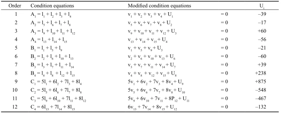
v= l – l) to the individual areas at this moment, the condi-tion equacondi-tions will be fulfilled exactly, which, regarding the system of calculations of closures, leads to the so-called modified condition equations (Table 3).

For the calculation procedure described below it is nec-essary to ensure linear independent conditions, that is why

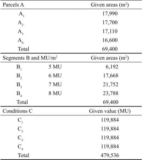
Table 1. Specification of the problem

Parcels A Given areas (m2_{) Segments of parcels Measured areas (m}2₎

A1 17,990 l1 2,641

A2 17,700 l2 4,698

A3 17,110 l3 5,530

A₄ 16,600 l₄ 5,082

Total 69,400 l5 2,481

Segments B and MU/m2 _{Given areas (m}2_{) l}

6 4,683

B1 5 MU 6,192 l7 5,319

B2 6 MU 17,668 l8 5,200

B3 7 MU 21,752 l9 1,049

B4 8 MU 23,788 l10 4,680

Total 69,400 l11 5,436

Conditions C Given value (MU) l12 6,005

C1 119,884 l13 3,547

C2 119,884 l14 5,506

C₃ 119,884 l₁₅ 7,491

C4 119,884 Total 69,348

Total 479,536

Table 2. Determination of the degrees of freedom

Number of observations n = 15

Number of necessary measurements k = 8

condition No. 8 in Table 3 was omitted in further calcula-tions as it is already included in the total sum of A type parcels and therefore it is redundant. For the assessment of the price of each A type parcel there are 4 additional conditions, but, analogically, one of them is redundant and has to be omitted (arbitrary one). For this reason condi-tion No. 12 was omitted in further calculacondi-tions. Thus the number of independent condition equations decreased to

s = 10. The system of equations is non-homogeneous due

to the unavoidable residues of areas.

The coefficients of corrections of the modified condition equations can be arranged into the so-called shape matrix

A. After notation

a₁ b₁ ... j₁

_a

2 b2 ... j2

A _{= : : . :} . . . an bn ... jn

it is possible to transform the system of equations into

the short form: AT_{v+ u = 0, where u =A}T_{l– u}

0, while

the elements of vector u₀ are the given areas and

pos-sibly the proposed values of the new parcels. It is not possible to directly figure out the individual unknowns as their number is higher than the number of equations. The problem would have an infinite number of solutions. According to Frobenius theorem, the system of equations has a solution if and only if the rank of the matrix of the system is equal to the rank of the augmented matrix of the system. Further to this, if the rank of the matrix of the system equals the number of unknowns, the system has only one solution. As in our case the number of unknowns

n = 15 and the rank of the matrix h(A) = 10, it would be

theoretically possible, in addition to the so-called basic

solution, to choose and a priori determine n – h(A) = 5

unknowns and to calculate the rest of them directly from the system of condition equations. Although the number of such selections is given by the combination number n 15

C_s (n) =

(

)

(

)

not all of the selections enable a unique solution. In order to obtain a unique solution we have to use an-other known relation for minimisation of the Euclidean metric:

_n

|| v || E = √ ∑pivi2 = min

i = 1

This function may be compared to criteria function known from optimisation tasks solved by mathemati-cal programming. If the matrix of weights is denoted as P = diag (p1, p2, ... , pn) , the minimum condition will be

in matrix notation:

vT_{Pv = min (2)}

The adjusted corrections of condition measurements may be calculated in various ways. A generalised

solu-tion of the LSM was presented e.g. by MÍKA (1985). The

simplest method of finding the minimum of a function, with the simultaneous satisfaction of further conditions, seems to be the calculation with the use of Lagrange coefficients.

The rule for the use of multiplicators was first published in 1788 by a French mathematician J. L. Lagrange in his Mécanique analytique for a wide class of tasks of the

calculus of variations – so-called Lagrange problems.

Lagrange wrote [quotation according to ALEXEJEV et al.

(1993)]: “It is possible to assert the following principle. If we are looking for the maximum or minimum of a func-tion of several variables with the condifunc-tion that there is a relation between these variables given by one or more equations, it is necessary to add to the minimised function the functions determining the equations of the relation, multiplied by indeterminate multiplicators and then look for the maximum or minimum of this sum as if the vari-ables were independent. The obtained equations together with the equations of the relations enable us to solve all the unknowns.”

According to the above-mentioned procedure, the system of the modified condition equations is multiplied in sequence by the so-far indeterminate Lagrange coeffi-cients (converted by multiplication -2 and called correlates

Table 3. Condition equations and modified condition equations

Order Condition equations Modified condition equations U_i

1 A1 = l1 + l2 + l3 + l4 v1 + v2 + v3 + v4 + U1 = 0 –39 2 A2 = l5 + l6 + l7 + l8 v5 + v6 + v7 + v8 + U2 = 0 –17 3 A3 = l9 + l10 + l11 + l12 v9 + v10 + v11 + v12 + U3 = 0 +60

4 A₄ = l₁₃ + l₁₄ + l₁₅ v₁₃ + v₁₄ + v₁₅ + U₄ = 0 –56

5 B1 = l1 + l5 + l9 v1 + v5 + v9 + U5 = 0 –21

according to C. F. Gauss) −2K_a, −2K_b, ... , −2K_j and added to the equation of the minimum condition. Thus the new “Lagrange function” is created:

Ω = vT_{Pv – 2k}T _(AT_{v + u) = min (3)}

To determine the minimum of this function it is neces-sary to partially differentiate it by the individual variables and then equate these derivations to zero in sequence:

∂Ω

––––– = 2Pv – 2Ak = 0 (4)

∂v

From the relation we can deduce the equations for

individual corrections: v = P–1_{Ak. These equations are}

then substituted into the modified condition equations and the result after rearrangement is the system of nor-mal equations for the calculation of unknown correlates. The arrangement of the equations in matrix notation is: AT_P–1_{Ak + u = 0 . Here it is possible to denote the matrix}

as N = AT_P–1_{A, where the matrix N is a symmetric matrix}

of coefficients of normal equations. The equations are in

the form Nk + u = 0 and their solutions are correlates

k = –N–1_u.

Subsequently the unknown correlates are calculated and from the equations of corrections it is also possible to calculate the individual v_i values. After substitution, the calculation with the weights is:

v = –P–1_{A (A}T_P–1_A)–1_{u (5)}

(without the necessity to quantify the k vector). Finally,

the adjusted values

l = l + v (6)

are calculated. The calculation is shown for example by BÖHM et al. (1990).

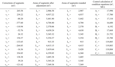
The adjusted values of corrections are presented for comparison in Table 4.

After the calculation of the adjusted segments of plots it

is possible to assess the a priori mean square error m₀ for

unit weight according to the known formulas: _vTPv

m₀ = ±

√

r

and the mean square errors of the individual measured quantities from the relation:

M2 _{= m}

02P–1 (8)

where: M = diag (m1, m2. ..., mn) – the matrix of the mean square errors,

M2 _{– the matrix of variances.}

In the case of adjustment with additional conditions, the calculated mean square errors characterise, rather than the accuracy of measurement, the correspondence of the proposed division (i.e. direction of the partitioning lines, proposed price of the divided plots) with the topology of the assignment and the extent of deformation of the input measurement. To evaluate the degree of this deformation, it is possible to calculate the ratio of the statistics τ with the use of:

a) measurement without additional conditions, b) including additional conditions.

In both cases, the same number of degrees of freedom

r = 7 is considered. The mentioned statistics are as

fol-lows:

a) If the presented problem is calculated without ad-ditional conditions, the apriori mean square error for

Corrections of segments

(m2₎ Areas of segments after _{adjustment (m}2₎ Areas of segments rounded _(m2₎

Control calculation of condition equations (m2_,

MU)

v1 = 265.58 L1 = 2,906.58 L1 = 2,907 A1 = 17,990

v2 = 239.22 L2 = 4,937.22 L2 = 4,937 A2 = 17,700

v3 = –88.20 L3 = 5,441.80 L3 = 5,442 A3 = 17,110

v4 = –377.60 L4 = 4,704.40 L4 = 4,704 A4 = 16,600

v5 = –110.94 L5 = 2,370.06 L5 = 2,370 B1 = 6,192

v6 = –52.76 L6 = 4,630.24 L6 = 4,630 B2 = 17,668

v7 = 26.32 L7 = 5,345.32 L7 = 5,345 B3 = 21,752

v8 = 154.37 L8 = 5,354.37 L8 = 5,354 B4 = 23,788

v9 = –133.65 L9 = 915.35 L9 = 915 C1 = 119,885

v10 = –264.85 L10 = 4,415.15 L10 = 4,415 C2 = 119,883

v11 = –16.36 L11 = 5,419.64 L11 = 5,420 C3 = 119,884

v12 = 354.85 L12 = 6,359.85 L12 = 6,360 C4 = 119,884

v13 = 138.38 L13 = 3,685.38 L13 = 3,685

v14 = 39.24 L14 = 5,545.24 L14 = 5,545

v15 = –121.62 L15 = 7,369.38 L15 = 7,369

unit weight (denoted by index a) is: m₀a _{= ± 0.346 (m}2₎

and the mean square error of the measurement of for example segment l₁ is: m₁a _{= ± 17.8 (m}2_).

b) If the presented problem is calculated with additional conditions, the a priori mean square error for unit

weight (denoted by index b) is: m₀b _{= ± 4.46 (m}2_{) and}

the mean square error of the measurement of for exam-ple segment l₁ is: m₁b _{= ± 229 (m}2_).

From the comparison of the mean square errors m₀b

τ_(apriori) = ––– = 12.9 (9)

m0a

it is possible to deduce to what extent the additional conditions worsened the calculated statistics and thus to express the degree of deformation that, in an ideal case,

should approach τ_(apriori) = 1. A more objective comparison

may be performed with the use of a posteriori statistics. For this purpose it is necessary to calculate the covariance

matrices of the adjusted measured quantities Ca _{and C}b_.

These matrices are calculated as:

C = m02 P–1(aposteriori) (10)

and the inversion weight matrix of the plot segments after adjustment is calculated as:

P–1

(aposteriori) = P–1 – P–1AN–1ATP–1 = P–1A(ATP–1A)–1ATP–1 (11)

Similar deduction is described for example in BÖHM

et al. (1990). The covariance matrixes are symmetric; the main diagonal elements contain the variances (squares of the mean square errors) while the off-diagonal elements contain covariances.

We choose a suitable criterion of optimality for assess-ment of the proposed solution. In relation to the previously described calculation of the ratio τ_(apriori), such a suitable criterion is the so-called A-optimality, as described e.g.

by PÁZMAN (1980) or KUBÁČEK and KUBÁČKOVÁ

(2000). A-optimality is defined by the calculation of the covariance matrix trace. The optimisation plan minimises

the scalar trC – trace of covariance matrix. This is in

fact minimisation of the Euclidean norm of the vector of a posteriori mean square values. On the other hand, the simplicity of calculation of this criterion is compensated by omission of the influence of the predicted covariances. It is possible to determine

√ tr1_C

τ_{(aposteriori)} = ––––– = 10.2 (12) √ tr2C

If there are more solutions to the division proposal, the better proposal in the sense of A-optimality will be the proposal with the lower τ_(apriori) or better τ_{(aposteriori)}.

For the sake of completeness it is possible to present the results of the calculation of a posteriori errors of the adjusted plot segments. For example, the mean square

error of the adjusted area of segment L₁ calculated

a) without additional conditions is

m₁a _{= ± 12.5 (m}2_),

b) from adjustment with additional conditions is

m₁b _{= ± 118 (m}2_).

RESULTS AND DISCUSSION

From the mathematical aspect, the minimising condi-tion of the LSM is expressed by the minimising condicondi-tion of the Euclidean norm (metrics) of a standardised vector

of corrections v. This method can be used in all cases

with excessive number of measurements, in this case of the redundantly measured segments of plots. If it is still possible to presume that the measured data show at least approximately normal distribution of probability, the use

of LSM is fully justified – see e.g.KUBÁČEK and PÁZMAN

(1979) or KUBÁČEK (1983). For the adjustment itself, the

question of error distribution makes no significant influ-ence. At the same time, the principle of adjustment of the condition measurements allows us to solve problems and closures of areas at intersections of various layers.

A sequel of previous as well as present legislative rules and rules for the administration of the cadastre documenta-tion and also rules for the preparadocumenta-tion of forest management plans admits the adjustment of areas, however, only in an rough way that can be applied to simple cases only. The adjustment of original areas of segments of evaluated soil-ecological units (ESEU) during division of agricultural land is not mentioned in the present cadastre rules at all.

This method can help solve such tasks of land division where the intersections of various layers of land registra-tion, evaluation and typological or price documentation occur. For example:

a) adjustment of areas of segments between parcels of real-estate cadastre and simplified records,

b) adjustment of areas of segments between parcels of real-estate cadastre and areas created by ESEU on agricul-tural land or areas of segments of GFT on forest land, c) adjustment of areas of segments between parcels of

real-estate cadastre and documentation for valuation with the use of added price conditions.

According to Act No. 344/1992, the areas in the cadastre documentation are recorded as rounded to integral square metres. Similarly, the calculation of forest valuation must show the same accuracy. If the adjustment of parcel segments was supposed to satisfy the additional price conditions even after rounding to integral MU, finding an integral solution with the use of other methods would be either impossible or, in the case of large systems of equa-tions, very difficult. For this purpose, after the calculation of LSM it is possible to apply some methods of discrete programming, such as the method of cutting hyperplanes in the calculation by the simplex method, branch and boundaries method and other methods, as summarised e.g. by PELIKÁN (2001). In practice, however, the solution of this discretisation problem is made significantly easier by the Decree to Property Valuation Act No. 540/2002, which sets down that the total price is rounded to 10 CZK.

The characteristics of the presented area adjustment can be summarised as follows:

determined as the reciprocal value of the corresponding area of adjusted segment.

b) Segments of areas can be adjusted by the method of adjustment of condition measurements, either by

in-determinate Lagrange coefficients (correlates) or by

adjustment of intermediary measurements. With re-spect to difficulty of the creation of normal equations (not always their number), the first method using the correlates is unambiguously more convenient. c) Functions determining the equations of adjustment

cor-rections are linear. In case they are not solved together with additional conditions, the coefficients of the shape

matrix A at the adjustment of the condition

measure-ments are equal either 0 or +1. In case that there are some additional (price) conditions, the coefficients in the respective condition equations agree with the valu-ation of the segment of the plot (in MU).

d) In case that the total adjusted area is equal in both boundaries of parcels from different layers (parcels are overlapping completely), in order to eliminate the possible singularity of the system of normal equations it is necessary to exclude redundant conditions and to

ensure that the linear vectors of the shape matrix A are

linearly independent.

e) As regards the preparation of various tasks of land divi-sion according to the previously set price, it is possible to supplement the condition equations with other – ad-ditional conditions, and then to adjust the areas with satisfaction of all these a priori conditions. The number of solved conditions must be lower than the number

of measurements n; in case it equals the number of

measurements n, it is not the case of adjustment.

f) The variation range of possible values of corrections is often determined in practice by the size of limit devia-tions in accordance with other standards and rules – for example Decree No. 84/1996 or Decree No. 190/1996. Using the standard procedures it is possible to deter-mine the accuracy characteristics of the quantities before and after valuation. In the case of valuation with

additional conditions, these statistics do not necessarily show the real accuracy of the input data, but they can still illustrate to what extent the proposed land divi-sion and evaluation are suitable from the typological aspect.

Acknowledgement

Thanks are due to Doc. Ing. FRANTIŠEK DOUŠEK, CSc.,

for guidance of this study.

References

ALEXEJEV V.M., TICHOMIROV V.M., FOMIN S.V., 1991. Matematická teorie optimálních procesů. Praha, Academia: 357.

BÖHM J., RADOUCH V., HAMPACHER M., 1990. Teorie chyb a vyrovnávací počet. Praha, GKP, 2 .vyd.: 416.

BUMBA J., 1992. Mapy velkých měřítek v České republice. Geodetický a kartografický obzor, 38/80 (12): 253–259. KUBÁČEK L., 1983. Základy teórie odhadu. Bratislava, Veda:

254.

KUBÁČEK L., KUBÁČKOVÁ L., 2000. Statistika a metrologie. Olomouc, Univerzita Palackého: 307.

KUBÁČEK L., PÁZMAN A., 1979. Štatistické metódy v meraní. Bratislava, Veda: 147.

MÍKA S., 1985. Numerické metody algebry. Praha, SNTL: 169.

PÁZMAN A., 1980. Základy optimalizácie experimentu. Bra-tislava, Veda: 180.

PELIKÁN J., 2001. Diskrétní modely v operačním výzkumu. Praha, Professional Publishing: 163.

VIŠŇOVSKÝ P., ČIHAL A., 1985. Geodézia a fotogrammetria. Bratislava, Príroda: 546.

ČÚZK, 2001. Návod pro správu a vedení katastru nemovitostí. Praha: 86.

Received for publication November 11, 2003 Accepted after corrections May 21, 2004

Využití variačního počtu pro dělení lesních pozemků

M. MATĚJÍK

Lesnická a dřevařská fakulta, Mendelova zemědělská a lesnická univerzita, Brno, Česká republika

ABSTRAKT:Příspěvek obsahuje využití metody nejmenších čtverců (MNČ) pro účely dělení a oceňování pozemků. Tuto metodu je možné použít všude tam, kde existuje nadbytečný počet měření, v tomto případě dílů ploch. Z matematického hlediska je mini-malizační podmínka MNČ jako normovaná podmínka ∑ pvv = min. , která minimalizuje euklidovskou normu ||v||_En-rozměrného vektoru reziduí dílů ploch za současného splnění daných podmínek. Výpočet je ukázán klasickým postupem variačního počtu pomocí Lagrangeovy funkce. Pokud jsou do výpočtu vloženy navíc další dodatečné podmínky, je možné na podkladě uvedených kritérií posoudit míru deformace zvoleného řešení na měřené veličiny.Využití metody vyrovnání podmínkových měření může pomoci řešit úlohy při dělení parcel na podkladě průniků vrstev parcel podle katastru nemovitostí a podle dřívějších pozemkových evidencí, bonitačních, typologických, cenových a jiných mapových podkladů.

Ocenění (hodnota) lesa se nejčastěji stanoví součtem hodnoty pozemku a hodnoty porostu. Grafickým podkla-dem pro výpočet ceny pozemku je vedle katastrální mapy mapa typologická, z níž se určí příslušnost dílu k soubo-ru lesních typů (SLT) a pro výpočet ceny porostu mapa porostní nebo obrysová. V případě současného ocenění lesních pozemků a lesních porostů a jejich rozdělení pod-le předem zadaného podílu je u navržené metody vhod-né, aby se nejprve průnikem typologické a porostní mapy vytvořily díly o stejném (konstantním) ocenění nejmenší plošné jednotky (cenová mapa) a teprve s těmito díly se pak dále pracovalo. Je tak možné lépe ztotožnit odpoví-dající si části hranic soborů lesních typů a jednotek pro-storového rozdělení lesa. Situaci je pak třeba porovnat se stavem pozemkové evidence – katastru nemovitostí.

Do výpočtu výměr se berou vždy všechny změnou do-tčené parcely. Součet jejich dosavadních výměr je inva-riantou, na kterou musí být výpočet výměr nového stavu – pokud rozdíl nepřekročí dopustnou mez – vyrovnán. Pro výpočet výměr parcel (a dílů) se používá ustálených způsobů, které jsou propracovány od nejstarších instrukcí a směrnic až po předpis ČÚZK (2001), platný v součas-né době. Ve složitějších případech průniků evidenčních nebo bonitačních vrstev jsou v nich uvedené jednoduché postupy vyrovnání nedostatečné a jejich aplikace může vést až k deformacím výměr řešené skupiny parcel.

Vyrovnané opravy podmínkových měření lze počítat různým postupem. Zobecněné řešení MNČ uvádí

na-příklad MÍKA (1985). Pro nalezení minima funkce za

současného splnění dalších podmínek je početně nejjed-nodušší výpočet pomocí Lagrangeových koeficientů.

V práci je řešena možnost využití variační metody na příkladu reálného rozdělení podílového spoluvlastnictví k lesnímu pozemku, jehož situace je zobrazena na obr. 1. Sestaví se soustava podmínkových rovnic, do nichž se dosadí měřené hodnoty. Soustava přetvořených podmín-kových rovnic se v klasickém řešení vynásobí po řadě zatím neurčitými součiniteli, Lagrangeovými koeficien-ty a sečte se s rovnicí podmínky minima. Utvoří se tak

nová „Lagrangeova funkce“ (3). Pro určení minima této funkce je nutné ji parciálně derivovat podle jednotlivých proměnných a tyto derivace postupně položit rovny nule (4). Vypočtou se hodnoty neznámých korelát a z rovnic

oprav se vypočtou jednotlivé hodnoty v_i. V rozepsaném

tvaru je výpočet s vahami (5). Nakonec se vypočtou vyrovnané hodnoty podle (6). Po výpočtu vyrovnaných

dílů ploch je možné stanovit apriorní střední chybu m₀

pro jednotkovou váhu a střední chyby jednotlivých mě-řených veličin ze vztahu (8); v maticovém vyjádření je

M matice středních chyb a M2 _{matice variancí. V}

pří-padě vyrovnání s dodatečnými podmínkami vypočítané střední chyby více než přesnost měření charakterizují to, zda navržený způsob dělení (např. směr dělících přímek, navrhovaná cena oddělených pozemků) odpovídá topo-logii zadání a do jaké míry vstupní měření deformuje. Pro posouzení míry této deformace je možné vypočítat poměr statistik τ pomocí:

a) měření bez dodatečných podmínek, b) včetně dodatečných podmínek.

Objektivnějším porovnáním je využití aposteriorních statistik. K tomu účelu je nutné vypočítat kovarianční

matice vyrovnaných měřených veličin Ca_{, C}b_{. Tyto}

ma-tice se vypočítají podle vzorce (10), přičemž inverzní

váhová matice P–1

(aposteriori) dílů ploch po vyrovnání se

vypočítá podle vzorce (11). Je možné určit vhodné kri-térium optimality pro posouzení zvoleného řešení. Ve

vztahu k uvedenému výpočtu poměru τ_(apriori) je takovým

vhodným kritériem tzv. A – optimalita, která je definová-na pomocí výpočtu stopy kovarianční matice.

Optimali-zační plán minimalizuje skalár trC – stopu kovarianční

matice. Jedná se vlastně o minimalizaci euklidovské nor-my vektoru aposteriorních středních chyb. Jednoduchost výpočtu tohoto kritéria je na druhé straně vyvážena tím, že neuvažuje vliv odhadnutých kovariancí. Je možné ur-čit τ_{(aposteriori)} podle (12). Pokud je k dispozici více řešení návrhu dělení, pak lepším návrhem ve smyslu A – opti-mality bude návrh s menším τ_(apriori) nebo lépe τ_{(aposteriori)}.

Corresponding author:

Ing. MIROSLAV MATĚJÍK, Mendelova zemědělská a lesnická univerzita, Lesnická a dřevařská fakulta, Lesnická 37, 613 00 Brno, Česká republika