Analysis of the efficiency of production processes became the focus of interest on the part of econo-mists in the 1950’s and this trend was initiated by the studies of Debreu (1951) and Farrell (1957), in which a measure of technical and overall efficiency of production was introduced. In the course of years, several analytical methods have been developed to evaluate technical efficiency. Many details on the early history of efficiency analysis may be found in an interesting study by Førsund and Sarafoglou (2002). These methods in terms of applied methodology rep-resent two fundamentally different approaches. The first one, i.e. the parametric approach, initiated by the studies of Aigner and Chu (1968), Timmer (1971) and Afriat (1972), uses the concept of the produc-tion funcproduc-tion and is based on a respectively modified regression analysis. It includes such methods as the corrected ordinary least squares (COLS), the modi-fied ordinary least squares (MOLS), or the stochastic frontier analysis (SFA). In turn, the other approach, i.e. the non-parametric one, in its mature form ap-peared slightly later, with a study by Charnes et al. (1978), and it is based on the solution of an adequately formulated problem of mathematical programming. In this respect, we need to mention several variants of the data envelopment analysis (DEA).
A considerable number of methods dealing with the same problem suggest a natural question on the
consistency of results obtained using different ana-lytical techniques based on an identical set of data. In such a situation, it is expected that all methods should lead to an identical or at least similar as-sessments of efficiency. However, it turns out that such a consistency is problematic. In the paper by Sharma et al. (1997), rather divergent estimates of technical efficiency were obtained. Similarly, in a study by Cubbin and Tzanidakis (1998), the authors showed that the application of the parametric and non-parametric approaches on the same data set can produce conflicting efficiency results.
The attempt to reduce the above mentioned dis-crepancies in the efficiency analysis has contributed to the creation of an intermediate method, combining the parametric and non-parametric approaches. Such a solution was proposed by Arnold et al. (1996). The suitability of such a combined approach was presented in the paper by Bardham et al. (1998), where the re-sults of extensive simulation studies were presented, which aim was mainly to evaluate the production function in the view of observations of many inef-ficient units. In simulation studies, the sample size is usually large and when generating observations, a previously established form of the production func-tion is used. In turn, in empirical investigafunc-tions the form of the production function is not known and the size of the sample frequently is not large. Thus it
On the combined estimation of technical efficiency and
its application to agriculture
Lucyna BŁAŻEJCZYK-MAJKA
1, Radosław KALA
21Department of Economic History, Adam Mickiewicz University in Poznań, Poznań, Poland 2Department of Mathematical and Statistical Methods, Poznań University of Life Sciences,
Poznań, Poland
Abstract: Assessment of effi ciency of businesses has been considered an object of interest by economists since the 1950’s. A number of methods have been developed, including the so-called parametric approaches, using the regression analysis, and the non-parametric approaches, connected with the mathematical programming techniques. However, the diversity of available methods, especially when supplying contradictory estimates, leads to confusion, hindering an objective interpre-tation of results. In this paper, we propose a procedure leading to the reduction of such discrepancies by the proper mo-difi cation of a combined method linking the non-parametric approach with a parametric one. Usefulness of the proposed solution is shown by estimation of technical effi ciency concerning the agricultural production in the USA and the selected regions of the European Union.
is still required to improve the estimation methods, so that reliable and objective estimates of efficiency may be obtained. This is possible after uncovering the sources of discrepancies and proposing methods of their elimination. The main aim of this study is to propose a new approach which combines and utilizes the strengths of the parametric and nonparametric methods. A special emphasis is placed on the sim-plicity of the analysis. Two empirical examples of the application of this proposed approach connected with the agricultural sector are presented, too.
MATERIAL AND METHODS
Parametric approaches
The main vehicle of parametric approaches is a production function. It reflects a direct relation be-tween inputs and usually a single output. Although the production function does not describe any particular production process, it mimics some processes in the sense that some inputs, represented here by a vector variable x, are indispensable in creating an output
y. Thus, the production function describes only the technological conditions of the production process. Usually, it is expressed in the form
y = f(x) = f(x; b)
where b is a vector of parameters characterizing the production technology of the given set of decision making units (DMUs).
The functional relation between inputs x and an output y should fulfil some obvious and some de-sirable requirements. The most obvious one states that x = 0 implies y = 0, i.e. f(0) = 0, and that f(x) is increasing in all inputs. The other conditions specify the functional form of f which reduces the choice to continuous, homogeneous and concave functions.
Probably the most popular in terms of the number of applications is the Cobb-Douglas production func-tion which, when the elasticity of scale is not greater than one, fulfils all the aforementioned requirements. Moreover, modelling with the Cobb-Douglas func-tion leads to simple models which are parsimonious in parameters having direct economical interpreta-tions. This feature is especially important when a set of DMUs is small. The next in popularity is the
translog production function, which, however, fulfils the basic requirements under very specific additional data dependent conditions.
A deterministic frontier production function is defined as the theoretical maximum output that a producer can obtain from the given vector of inputs. Having chosen the form of the frontier production function y = f(x), the output oriented technical ef-ficiency is measured by the quotient TE = y/f(x) ≤ 1. This quantity, referred to the i-th unit which pro-duces an output yi from a vector xi of inputs, can be interpreted as the factor rescaling the value of the frontier production function to obtain the actual level of output, i.e. yi = f(xi)TEi.
The simplest way of establishing the frontier pro-duction function is the COLS method. It is performed in two steps. First, using the observations (yi, xi), i = 1, 2, …, n, of the given set of DMUs, the estimate of
f(x; b) is evaluated. It can be done by the ordinary least squares regression, because the production function is usually linear in the logs of the variables. Then, the resulting function ln f(x; b) is shifted upwardly with respect to the largest positive residual a = max(ei). In consequence, the log of the frontier production function has the form
ln f(x) = ln f(x;b) + a
and
TEi(a) = exp(ln yi – ln f(xi)) = exp(–ui)
where ui = a – ei ≥ 0 is the measure of the output-oriented technical inefficiency in the COLS method.
The shifting term may also be chosen according to a different rule, taking into account some specific as-sumptions about the distribution of ui. If it is assumed that they follow an exponential distribution, then ln f(x; b) should be shifted by the standard deviation of residuals, sD, following from the regression analysis (e.g. Greene 2008: 106). This is the simplest variant of the MOLS method. In such a case, however, not all estimated inefficiency measures are positive, since
sD < max(ei). As a result, some units can appear to be technically over-efficient. These over-efficiencies may be caused by some specific conditions of the production process, which were beyond the control of the DMUs. Therefore, to preserve the sense of the technical efficiency concept, the over-efficiency must be truncated, i.e. TEi(sD) = min{exp(–sD + ei), 1}.
Note, moreover, that rescaling all exp(–sD + ei),
An idea of incorporating into the model the con-ditions not controlled by the DMUs resulted in the stochastic frontier analysis (SFA). In this approach, initiated by Aigner et al. (1977) and Meeusen and van den Broeck (1977), the frontier production func-tion, contrary to the previous deterministic case, is assumed to be stochastic,
y = f(x)exp(v)
where v is a random variable representing distur-bances that are not dependent on the DMUs. To obtain the level of the output observed, it must be again rescaled by an additional term TE = exp(–u), where
u is now a nonnegative random variable represent-ing the technical inefficiency. In consequence, the stochastic frontier production function is estimated in presence of the standard disturbance term v, as in the regression model, and the technical inefficiency
u, the latter term introducing into the model some additional and specific assumptions concerning the form of the probability distribution. The change in the form of the frontier production function, which is now a random variable, also causes a change in the understanding of the measure of the technical efficiency. In the stochastic approach, it is related with the quotient of two conditional expected values, TE = E(y|u)/E(y|u = 0) (e.g. Battese and Coelli 1992). The expectation E(y|u) represents the averaged level of output y (averaged with respect to the conditions not controlled by the producer), while E(y|u = 0) also represents the averaged output y, but for the produc-tion process being technically the most efficient.
Non-parametric approaches
The main idea of non-parametric approaches fo-cuses on formulating a series of appropriate linear programming problems, in which the most efficient producers are identified in the observed set of DMUs. This idea, first pointed out by Farrell (1957), was fully elaborated by Charnes et al. (1978) and since then it has been known as the data envelopment analysis (DEA). In this method, the efficiency of each producer is evaluated with respect to the given group of them, by comparing the observed outputs and vectors of inputs characterizing all producers under investigation.
A particular formulation of the linear program depends on the initial assumptions. They concern the type of orientation, which can be focused on the
outputs maximization given the values of inputs, or on the inputs minimization given the values of outputs, and the type of technology restrictions, which can be the constant returns to scale (CRS) or the variable returns to scale (VRS). Many other formulations of the DEA are reviewed by Thanassoulis et al. (2008) (see also Coelliet al. 2005; Cooper et al. 2007).
In the case of a single output oriented DEA, which corresponds to the considerations of Section 2, and under the CRS assumption, an estimate of the techni-cal efficiency of the i-th producer follows by solving a linear program of the form:
Maxq,l q, subject to: –qyi + yλ ≥ 0, xi – Xλ ≥ 0, λ ≥ 0
where yi and xi represent the output and the vector of inputs, respectively, of the i-th unit, while y and
X are the vector of outputs and the matrix of inputs, respectively, of all producers in the sample. The score of technical efficiency of the i-th unit is the inverse of solution θ, TEci = 1/θ. When TEci is equal to one, the i-th producer is a frontier, i.e. the most efficient producer in the whole set of the DMUs.
When the CRS restriction is replaced by the VRS, the above formulated linear program changes by adding the condition that all λ’s sum to one. This convexity constraint envelops the data set more tightly, which now is covered by the convex hull rather than the convex cone only, as in the case of the CRS. In con-sequence, the corresponding estimate of the technical efficiency TEvi is not less than TEci for each DMU.
Th e results of the DEA procedures are often employed as the dependent variable in the further analysis search-ing socioeconomics sources of diff erences between the units’ effi ciency (Assaf and Matawie 2009; Hu et al. 2009; Olson and Vu 2009; Assaf and Agbola 2011). However when comparing the non-parametric approaches with those based on the regression analysis (RA), which are presented in Section 2, the diff erences between them are easily visible. Th e RA methods require many specifi c assumptions concerning the form of the production function as well as they are related with the type of the probability distributions of random variables involved in the model. Moreover, the estimation of unknown parameters and effi ciency scores is possible when the sample size, i.e. the set of the DMUs, is large, which is especially important for the SFA.
in-efficiency, which are related exactly with the set of DMUs under considerations. Some other differ-ences between these two techniques are discussed by Cubbin and Tzanidakis (1998) and Sena (2003). These authors observed also that the DEA and RA approaches may give very different results. The other arguments supporting this observation can be found in papers by Ferrier and Lovell (1996), Sharma et al. (1997) as well as Sahoo et al. (1999).
The combined approach and its modification
In the paper by Arnold et al. (1996), a combined method of estimating the production function was proposed. This method is accomplished in two stages. First, the DEA is used to identify the frontiers in a set of DMUs. Next, the RA with a selected form of the production function is applied to all DMUs, but the regression model is supplemented by a dummy variable distinguishing between the efficient and inefficient units. In consequence, two production functions, for the frontiers and non-frontiers, are established. Having estimated the frontier produc-tion funcproduc-tion, the estimates of the technical effi-ciencies of all DMUs may be obtained. Of course, some truncations of over-efficiency of some units are necessary. We will furthermore denote this ap-proach as the DE+RA.
The method presented above, however, does not guarantee that the efficiencies obtained will be in full agreement with that following from the DEA. Although small differences may be easily explained by the differences in the computational procedures, large disagreements, if they take place, must have more severe causes. At this point, first of all note that the definitions of technical efficiency in the case of stochastic and deterministic frontier production functions are different, which causes difficulty in a direct comparison of efficiencies following from the SFA with those following from the other approaches. As to comparisons between the non-parametric approaches and those based on the deterministic frontier production function, it should be noted that in general the model assumptions of the RA, of the DEA(CRS) and of the DEA(VRS) are different. In consequence, they will produce different esti-mates of technical efficiencies for the same data set. They will provide similar results only in special cases. Since the CRS assumption corresponds with the linear homogeneity of production function, we
can expect similar efficiencies following from the DEA(CRS) and the standard regression approaches. They will be very close, if the data actually support this specific assumption. The question appears what if it is not the case.
If the condition of constant returns to scale is not satisfied, then the DEA(VRS) may produce efficiencies much more different from those following from the RA. To explain this, note that the VRS output ori-ented linear program, as observed by Pastor (1996), is invariant with respect to any translation of the input vectors, provided that the shift is the same for all DMUs. It is not a property of the production function, since by the standard assumptions, it is increasing in all inputsand f(0) = 0. These assumptions imply in particular that even small non-zero inputs lead to a positive quantity of an output, while in practice, to obtain a positive amount of the output, some critical non-zero, unfortunately unknown, quantities of all inputs are necessary. This divergence can be reduced by a proper translation of the production function, i.e. by subtracting from the input vector x some vec-tor δ of positive constants. Note that a shift of the production function from f(x;β) to f(z;β), where z =
x – δ, does not change its shape. Of course, the role of the parameter vector β is not the same in both cases, and some attention should be paid when interpreting parameters in the economic sense.
In consequence, the resulting frontier production function f(z;b) enables the estimation of technical efficiencies of all DMUs. This method will be denoted by the DE+RAs.
Finally, note that the equation f(x) = f(z) implies the equality of the corresponding partial derivatives, which means that the marginal efficiencies following from both functions are the same. It is not in the case of elasticities. However, for the j-th input they can be simply recalculated as follows:
j j j j
j j
z x z f
x x f
x ( )
) ( ) ( )
(
x x
where zj = xj – δj. Summing up elasticities e(xj) over all inputs, the elasticity of scale can be obtained. Note also that here elasticity ε(xj) is a function of xj, even in the case of the Cobb-Douglas production function.
Data
To illustrate the considerations of the previous sections, we will examine two data sets. The first one concerns the production in the year 2001 of 34 regions from Belgium (1 region), France (22), The Netherlands (1), Luxemburg (1) and the western part of Germany (9). The data were taken from the Farm Accounting Data Network. The value of the total agriculture production was used as the output variable. As the input variables, we had initially se-lected total the utilized agricultural area, labour and materials, but the first variable, land, appeared to be insignificant and was eliminated from the analysis.
In the second example, we used the data set which was analysed by Farrell (1957) when he introduced the main idea of the DEA approach. This data set characterizes the agriculture production in the United States in the year 1952. Farrell has estimated the technical efficiencies of 48 states using, in particular, cash receipts from farming, with the home consump-tion included, as the output, and various sets of input variables. In particular, he used the following: land, labour and materials.
Technical efficiencies were calculated by two nonparametric methods, the DEA(CRS) and the DEA(VRS), two regression methods, the COLS and MOLS, the combined method DE+RA and the pro-posed one, the DE+RAs, with a shift of input vectors. In parametric approaches as well as in the combined ones we used the Cobb-Douglas function, which en-sures the smallest number of free parameters.
RESULTS
Estimates of technical efficiencies for the first data set related to the EU agriculture are presented in Table 1. In the last columns, the elasticity of labour and materials as well as of scale are contained. They were calculated using the proposed DE+RAs method. The averages of these elasticities,
ε(labour) = 0.145, ε(materials) = 0.992, ε(scale) = 1.137
indicate that the second input, materials, is the most effective and that the constant returns to scale as-sumption is disturbed.
The last two rows of Table 1 present Pearson’s coef-ficients of correlation between the results following from the non-parametric and the remaining methods. The correlation between efficiencies obtained from DEA(CRS) and DEA(VRS) is not very high, which means that the constant returns to scale assumption significantly influences the resulting efficiencies. On the other hand, observe quite a high correla-tion between efficiencies following from DEA(VRS) with those following from DE+RAs, which is in har-mony with the established scale elasticity 1.137 > 1. Moreover, observe very high correlations between results of the DEA(CRS) and of COLS, and of MOLS, which means that in these methods the elasticity of scale is near to one. Indeed, the estimated logs of this function are as follows:
COLS: log f (x) = 0.563 + 0.127 log x1 + 0.907 log x2
(0.581) (0.022) (0.052) ε (scale) = 1.034 (0.051) R2 = 0.929
MOLS: log f (x) = 0.475 + 0.127 log x1 + 0.907 log x2 (0.581) (0.022) (0.052)
ε(scale) = 1.034 (0.051)
where x1 here represents labour, x2 denotes mate-rials, R2 the coefficient of determination, while in
parentheses the standard deviations of estimated parameters are given.
On the other hand, frontier production functions fol-lowing from the combined approaches take the forms:
DE+RA: log f (x) = –0.573 + 0.146 log x1 + 0.983 log x2
(0.637) (0.022) (0.057)
ε(scale) = 1.130 (0.057) R2 = 0.952
DE+RAs: log f (z) = 3.893 + 0.126 log z1 + 0.636 log z2
where z1 = x1 – 53.18, z2 = x2 –33420.60. The transla-tion vector δ in the DE+RAs method was equal to 60% of the vector (88.63, 55701.00) composed from the minimal values of both inputs. The minimal shift in the case of labour is not less than 2% (of the maximal observed labour), while in the case of materials it is not less than 15% (of the maximal observed value of materials). Thus the shift with respect to the second variable was much more restrictive. Note also that the frontier production function f(x) following from DE+RA is convex, while that with shifted input
vari-ables f(z), estimated by the DE+RAs method, and is concave as required. Comparing both methods we can notice that the proposed one provides efficien-cies compatible with that following from the non-parametric DEA (VRS) approach.
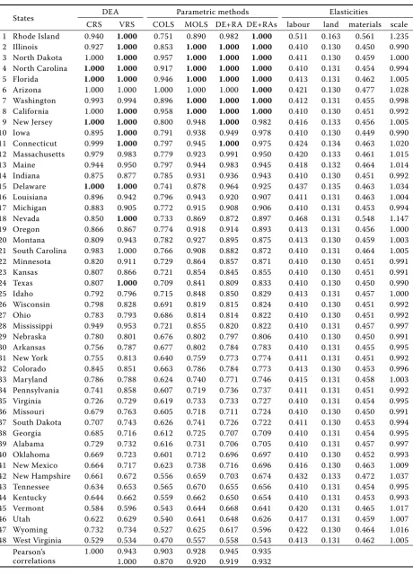
[image:6.595.69.531.270.743.2]The estimated efficiencies from the second data set related to the USA agriculture are contained in Table 2. This table is organized in the same way as the previous one, with the exception that now we have three inputs: land (x1), labour (x2) and materials (x3).
Table 1. Estimates of technical efficiencies of agricultural production in 34 regions of EU
Regions DEA Parametric methods Elasticity’s
CRS VRS COLS MOLS DE+RA DE+RAs labour materials scale
1 Belgium (BEL) 1.000 1.000 1.000 1.000 1.000 1.000 0.139 0.898 1.037
2 Hamburg (DEU) 1.000 1.000 0.951 1.000 1.000 1.000 0.131 0.955 1.086
3 Bayern (DEU) 0.945 1.000 0.899 0.982 1.000 1.000 0.163 1.121 1.284
4 Saarland (DEU) 1.000 1.000 0.941 1.000 1.000 1.000 0.316 0.930 1.246
5 Languedoc-Roussillon (FRA) 0.911 1.000 0.871 0.952 1.000 1.000 0.132 1.396 1.528
6 Provence-Apes-Côte (FRA) 1.000 1.000 0.950 1.000 1.000 1.000 0.129 1.108 1.238
7 The Netherlands (NED) 0.950 1.000 0.895 0.977 0.928 1.000 0.130 0.749 0.879
8 Champagne-Ardenne (FRA) 0.987 1.000 0.940 1.000 1.000 0.997 0.132 0.858 0.989
9 Corse (FRA) 0.825 1.000 0.795 0.869 0.930 0.996 0.133 1.589 1.722
10 Franche-Comté (FRA) 0.948 0.962 0.887 0.968 1.000 0.960 0.158 0.961 1.118
11 Auvergne (FRA) 0.844 1.000 0.809 0.884 0.963 0.956 0.169 1.289 1.458
12 Alsace (FRA) 0.918 0.967 0.886 0.968 1.000 0.953 0.134 1.037 1.171
13 Limousine (FRA) 0.770 1.000 0.761 0.832 0.912 0.949 0.163 1.490 1.653
14 Rheinland-Pfalz (DEU) 0.903 0.968 0.869 0.949 0.989 0.946 0.134 1.093 1.227
15 Bretagne (FRA) 0.906 0.946 0.883 0.965 0.960 0.946 0.134 0.825 0.959
16 Rhônes-Alpes (FRA) 0.887 0.959 0.854 0.933 0.974 0.933 0.134 1.108 1.243
17 Niedersachsen (DEU) 0.872 0.924 0.865 0.945 0.953 0.922 0.137 0.852 0.989
18 Hessen (DEU) 0.876 0.906 0.835 0.912 0.966 0.912 0.155 1.028 1.183
19 Schleswig-Holstein (DEU) 0.870 0.899 0.852 0.930 0.931 0.909 0.135 0.838 0.973
20 Baden-Württemberg (DEU) 0.864 0.901 0.838 0.915 0.947 0.896 0.135 0.999 1.134
21 Nordrhein-Westfalen (DEU) 0.858 0.865 0.839 0.917 0.926 0.891 0.135 0.872 1.008
22 Nord-Pas-de-Calais (FRA) 0.845 0.906 0.835 0.912 0.921 0.891 0.138 0.852 0.990
23 Basse-Normandie (FRA) 0.869 0.875 0.834 0.911 0.938 0.890 0.144 0.901 1.045
24 Pays de la Loire (FRA) 0.837 0.837 0.832 0.909 0.928 0.884 0.138 0.898 1.036
25 Lorraine (FRA) 0.871 1.000 0.797 0.871 0.885 0.865 0.151 0.828 0.979
26 Luxembourg (LUX) 0.819 0.836 0.804 0.879 0.897 0.857 0.140 0.884 1.025
27 Aquitaine (FRA) 0.852 0.858 0.807 0.882 0.891 0.854 0.131 0.941 1.071
28 Picardie (FRA) 0.805 0.909 0.787 0.860 0.847 0.852 0.134 0.798 0.932
29 Midi-Pyrénées (FRA) 0.762 0.876 0.752 0.822 0.870 0.837 0.140 1.159 1.299
30 Bourgogne (FRA) 0.809 0.809 0.786 0.859 0.874 0.833 0.135 0.909 1.043
31 Poitou-Charentes (FRA) 0.775 0.817 0.776 0.848 0.881 0.831 0.141 0.977 1.118
32 Haute-Normandie (FRA) 0.760 0.813 0.751 0.820 0.829 0.801 0.138 0.853 0.991
33 Île de France (FRA) 0.727 0.741 0.689 0.753 0.747 0.732 0.131 0.845 0.976
34 Centre (FRA) 0.710 0.715 0.681 0.743 0.749 0.720 0.133 0.884 1.017
Pearson’s correlations
1.000 0.759 0.974 0.965 0.870 0.851
1.000 0.728 0.744 0.813 0.925
Table 2. Estimates of technical efficiencies of agricultural production in the United States
States DEA Parametric methods Elasticities
CRS VRS COLS MOLS DE+RA DE+RAs labour land materials scale
1 Rhode Island 0.940 1.000 0.751 0.890 0.982 1.000 0.511 0.163 0.561 1.235
2 Illinois 0.927 1.000 0.853 1.000 1.000 1.000 0.410 0.130 0.450 0.990
3 North Dakota 1.000 1.000 0.957 1.000 1.000 1.000 0.411 0.130 0.459 1.000
4 North Carolina 1.000 1.000 0.917 1.000 1.000 1.000 0.410 0.131 0.454 0.994
5 Florida 1.000 1.000 0.946 1.000 1.000 1.000 0.413 0.131 0.462 1.005
6 Arizona 1.000 1.000 1.000 1.000 1.000 1.000 0.421 0.130 0.477 1.028
7 Washington 0.993 0.994 0.896 1.000 1.000 1.000 0.412 0.131 0.455 0.998
8 California 1.000 1.000 0.958 1.000 1.000 1.000 0.410 0.130 0.451 0.992
9 New Jersey 1.000 1.000 0.800 0.948 1.000 0.982 0.416 0.133 0.456 1.005
10 Iowa 0.895 1.000 0.791 0.938 0.949 0.978 0.410 0.130 0.449 0.990
11 Connecticut 0.999 1.000 0.797 0.945 1.000 0.975 0.424 0.134 0.463 1.020
12 Massachusetts 0.979 0.983 0.779 0.923 0.991 0.950 0.420 0.133 0.461 1.015
13 Maine 0.944 0.950 0.797 0.944 0.983 0.945 0.418 0.132 0.464 1.014
14 Indiana 0.875 0.877 0.785 0.931 0.936 0.943 0.410 0.130 0.451 0.992
15 Delaware 1.000 1.000 0.741 0.878 0.964 0.925 0.437 0.135 0.463 1.034
16 Louisiana 0.896 0.942 0.796 0.943 0.920 0.907 0.411 0.131 0.463 1.004
17 Michigan 0.883 0.905 0.772 0.915 0.908 0.906 0.410 0.131 0.453 0.994
18 Nevada 0.850 1.000 0.733 0.869 0.872 0.897 0.468 0.131 0.548 1.147
19 Oregon 0.866 0.867 0.774 0.918 0.914 0.893 0.413 0.131 0.456 1.000
20 Montana 0.809 0.943 0.782 0.927 0.895 0.875 0.413 0.130 0.459 1.003
21 South Carolina 0.983 1.000 0.766 0.908 0.882 0.872 0.410 0.131 0.464 1.005
22 Minnesota 0.820 0.911 0.729 0.864 0.857 0.871 0.410 0.130 0.451 0.991
23 Kansas 0.807 0.866 0.721 0.854 0.845 0.855 0.410 0.130 0.451 0.991
24 Texas 0.807 1.000 0.709 0.841 0.809 0.833 0.410 0.130 0.450 0.990
25 Idaho 0.792 0.796 0.715 0.848 0.850 0.829 0.413 0.131 0.457 1.000
26 Wisconsin 0.798 0.828 0.691 0.819 0.815 0.824 0.410 0.130 0.451 0.992
27 Ohio 0.783 0.793 0.686 0.814 0.814 0.822 0.410 0.130 0.451 0.992
28 Mississippi 0.949 0.953 0.721 0.855 0.820 0.822 0.410 0.131 0.457 0.997
29 Nebraska 0.780 0.801 0.676 0.802 0.797 0.806 0.410 0.130 0.450 0.991
30 Arkansas 0.756 0.787 0.677 0.802 0.784 0.783 0.410 0.131 0.455 0.995
31 New York 0.755 0.813 0.640 0.759 0.773 0.774 0.411 0.131 0.451 0.992
32 Colorado 0.845 0.851 0.663 0.786 0.784 0.773 0.413 0.130 0.453 0.996
33 Maryland 0.786 0.788 0.624 0.740 0.771 0.746 0.415 0.131 0.458 1.003
34 Pennsylvania 0.741 0.858 0.607 0.719 0.736 0.737 0.411 0.131 0.451 0.992
35 Virginia 0.726 0.729 0.619 0.733 0.733 0.727 0.410 0.131 0.454 0.995
36 Missouri 0.679 0.763 0.605 0.718 0.711 0.724 0.410 0.130 0.450 0.991
37 South Dakota 0.707 0.743 0.626 0.741 0.726 0.722 0.411 0.130 0.453 0.994
38 Georgia 0.685 0.716 0.612 0.725 0.707 0.709 0.410 0.131 0.454 0.995
39 Alabama 0.729 0.732 0.616 0.731 0.706 0.705 0.410 0.131 0.457 0.997
40 Oklahoma 0.669 0.723 0.601 0.712 0.696 0.697 0.410 0.130 0.452 0.993
41 New Mexico 0.664 0.717 0.623 0.738 0.716 0.696 0.416 0.130 0.463 1.009
42 New Hampshire 0.661 0.672 0.556 0.659 0.703 0.674 0.432 0.133 0.472 1.037
43 Tennessee 0.634 0.653 0.565 0.670 0.655 0.656 0.410 0.131 0.454 0.995
44 Kentucky 0.644 0.662 0.559 0.662 0.650 0.654 0.410 0.131 0.453 0.993
45 Vermont 0.584 0.596 0.543 0.644 0.668 0.641 0.420 0.131 0.465 1.017
46 Utah 0.622 0.629 0.540 0.641 0.648 0.626 0.417 0.131 0.459 1.007
47 Wyoming 0.732 0.734 0.527 0.625 0.617 0.596 0.422 0.130 0.464 1.016
48 West Virginia 0.529 0.534 0.470 0.557 0.558 0.543 0.413 0.131 0.462 1.005
Pearson’s correlations
1.000 0.943 0.903 0.928 0.945 0.935
1.000 0.870 0.920 0.919 0.932
First of all, it needs to be noted that the averaged elasticity of scale, 1.010, corresponds perfectly to that assumed by Farrell, who used the constant re-turns to scale Cobb-Douglas function. The averaged elasticities of inputs,
ε (labour) = 0.417, ε (land) = 0.132, ε(materials) = 0.461
also correspond to those calculated by Farrell. The main advantage of parametric approaches, however, is a possibility of establishing the form of the frontier production function. The estimated logs of this function, obtained in the frames of models under considerations, are as follows:
COLS:
log f (x) = –2.180 + 0.406 log x1 + 0.112 log x2 + 0.492 log x3
(0.581) (0.040) (0.025) (0.045) ε(scale) = 1.010 (0.026) R2 = 0.974
MOLS:
log f (x) = –2.174 + 0.406 log x1 + 0.112 log x2 + 0.492 log x3
(0.581) (0.040) (0.025) (0.045) ε(scale) = 1.010 (0.026) R2= 0.974
DE+RA:
log f (x) = 1.113 + 0.426 log x1 + 0.134 log x2 + 0.463 log x3
(0.477) (0.056) (0.031) (0.052) ε(scale) = 1.023 (0.028) R2 = 0.985
DE+RAs:
log f (z) = –1.842 + 0.409 log z1 + 0.130 log z2 + 0.449 log z3
(0.460) (0.054) (0.030) (0.051) ε(scale) = 1.009 (0.006) R2 = 0.985
where z1 = x1 – 0.39, z2 = x2 – 11.87, z3 = x3 – 859.94.
In the DE+RAs method the translation vector was equal to 20% of the vector (1.97, 59.36, 4299.72) composed from the minimal values of all the three inputs. This time the translation was rather small. In consequence, the differences between the coef-ficients of functions following from the combined methods are almost indistinguishable. Moreover, they are also very similar to those following from the COLS and MOLS approaches. This agreement is a consequence of the constant return to scale as-sumption, which is strongly supported by the data. It is confirmed by a very high correlation coeffi-cient between results obtained from DEA(CRS) and DEA(VRS). In consequence, we have also very high correlations between efficiencies following from the other methods. Nevertheless, technical efficiencies produced by the proposed DA+RAs method are most similar to those following from the non-parametric DEA(VRS).
CONCLUSIONS
In the paper various techniques of evaluating techni-cal efficiency are discussed. Among them we consid-ered the non-parametric approaches related with data envelopment analysis (DEA), parametric ones based on regression analysis (RA) and using the concept of frontier production function, and the combined method linking both parametric and non-parametric approaches. Unfortunately, different methods, as it was observed by some authors, can produce very dif-ferent estimates of efficiencies, which is unexpected when analysing the same data set. Therefore, in the presentation of various methods we paid special at-tention to their differences and weak points in the context of technical efficiency estimation.
In this respect we noted that in the case of stochastic frontier functions and deterministic frontier func-tions there is an important difference in the defini-tions of technical efficiency. This justifies even large differences between estimated efficiencies, since the crucial assumptions of these models are different. In turn, we have observed that the DEA approach can deliver similar estimates as the RA approach with a deterministic production function, but only if the basic assumptions of the methods applied are consistent and simultaneously these assumptions are supported by the data under investigation. As a result of this discussion we have proposed a shift of the produc-tion funcproduc-tion, which modificaproduc-tion may improve the estimation process in a case when the assumption of constant returns to scale is not valid. The usefulness of this modified method is illustrated by analyses of two data sets concerning agricultural production.
REFERENCES
Aigner D.J., Chu S.F. (1968): On estimating the industry production function. American Economic Review, 58: 226–239.
Aigner D., Lovell K., Schmidt P. (1977): Formulation and estimation of stochastic frontier production function models. Journal of Econometrics, 6: 21–37.
Afriat S. (1972): Efficiency estimation of production func-tion. International Economic Review, 13: 568–598. Arnold V.L., Bardham I.R., Cooper W.W., Kumbhakar S.C.
Assaf A.G., Agbola F.W. (2011): Modeling the performance of Australian hotels: a DEA double bootstrap approach. Tourism Economics, 17: 73–89.
Assaf A.G., Matawie K.M. (2009): A two-stage approach to efficiency modeling: an application to the Australian hospital food production industry. Journal of Hospitality & Tourism Research, 33: 284–304.
Battese G.E., Coelli T.J. (1992): Frontier production func-tion. Technical efficiency and panel data: with applica-tions to paddy farmers in India. Journal of Productivity Analysis, 3: 153–169.
Bardham I.R., Cooper W.W., Kumbhakar S.C. (1998): A simulation study of joint uses of data envelopment analy-sis and statistical regressions for production function estimation and efficiency evaluation. Journal of Pro-ductivity Analysis, 9: 249–278.
Charnes A., Cooper W.W., Rhodes E. (1978): Measuring the efficiency of decision making units. European Journal of Operational Research, 2: 429–444.
Coelli T.J., Rao D.S.P., O’Donnell C .J., Battese G.E . (2005): An Introduction to Efficiency and Productiv-ity Analysis.2nd ed. Springer Science+Business Media,
New York.
Cooper W.W., Seiford L.M., Tone K. (2007): Data Envel-opment Analysis: A Comprehensive Text with Models, Applications, References and Dea-solver Software. 2nd
ed. Springer Science+Business Media, New York. Cubbin J., Tzanidakis G. (1998): Regression versus data
envelopment analysis for efficiency measurement: an application to the England and Wales regulated water industry. Utilities Policy, 7: 75–85.
Debreu G. (1951): The coefficient of resource utilization. Econometrica, 19: 14–22.
Ferrier G.D., Lovell C.A.K. (1996): Measuring cost effi-ciency in banking. Journal of Econometrics, 46: 229–245. Farrell M.J. (1957): The measurement of productive ef-ficiency of production. Journal of the Royal Statistical Society, Series A, 120(III): 253–281.
Førsund F.R., Sarafoglou N. (2002): On the origins of data envelopment analysis. Journal of Productivity Analysis, 17: 23–40.
Greene W.H. (2008): The econometric approach to ef-ficiency analysis. In: Fried H., Lovell K., Schmidt S. (eds): The Measurement of Productive Efficiency and Productive Growth. Oxford University Press, Oxford New York.
Hu J.L., Shieh H.S., Huang C.H., Chiu C.N. (2009): Cost efficiency of international tourist hotels in Taiwan: a DEA application. Asia Pacific Journal of Tourism Re-search, 14: 371–384.
Meeusen W., van den Broeck J. (1977): Efficiency estimation from Coob-Douglas production function with composed errors. International Economic Review, 18: 435–444. Olson K., Vu L. (2009): Economic efficiency in farm
house-holds: trends, explanatory factors, and estimation meth-ods. Agricultural Economics, 40: 587–599.
Pastor J. T. (1996): Translation invariance in data envelop-ment analysis: A generalization. Annals of Operations Research, 66: 93–102.
Sahoo B. K., Mohapatra P. K. J., Trivedi M. L. (1999): A comparative application of data envelopment analysis and frontier translog production function for estimating returns to scale and efficiencies. International Journal of System Sciences, 30: 379–394.
Sena V. (2003): The frontier approach to the measurement of productivity and technical efficiency. Economic Is-sues, 8: 71–97.
Sharma K.R, Leung P., Zaleski H.M. (1997): Productive efficiency of the swine industry in Hawaii: stochastic frontier vs. data envelopment analysis. Journal of Pro-ductivity Analysis, 8: 447–459.
Thanassoulis E., Portela M., Despić O. (2008): Data en-velopment analysis: the mathematical programming approach to efficiency analysis. In: Fried H., Lovell K., Schmidt S. (eds): The Measurement of Productive Efficiency and Productive Growth. Oxford University Press, Oxford, New York.
Timmer P. (1971): Using a probabilistic frontier produc-tion funcproduc-tion to measure technical efficiency. Journal of Political Economy, 79: 776–794.
FAND data. Available at http://ec.europa.eu/agriculrure/ rica
Received: 23th May 2014
Accepted: 20th January 2015
Contact address:
Lucyna Błażejczyk-Majka, Department of Economic History, Adam Mickiewicz University in Poznań, ul. Św. Marcin 78, 61-809 Poznań, Poland

![A Molecular Electron Density Theory Study of the Reactivity of Azomethine Imine in [3+2] Cycloaddition Reactions](data:image/gif;base64,R0lGODlhAQABAIAAAP///wAAACH5BAEAAAAALAAAAAABAAEAAAICRAEAOw==)