The rheological properties of cheeses are significantly connected with their final quality (KFOURY et al. 1989). Like most of solid biological materials cheeses exhibit the viscoelastic behaviour. This means that their behav-iour under some mechanical loading consists of solid (elastic) and fluid (viscous) behaviour. The viscoelastic materials are those in which the relationship between stress and strain depends on time. There are many models of the viscoelastic behaviour of materials, see e.g. LAKES (1999) for a review. The choice of a viscoelastic model and the evaluation of its parameters is based on the use of some phenomena which occur in viscoelastic materials. The main phenomena are:
– Creep – if the stress is held constant, the strain increa-ses with time;
– Relaxation – the stress decreases with time at constant strain;
– The effective stiffness depends on the rate of load ap-plication;
– If cyclic loading is applied, hysteresis occurs; – Acoustic waves experience damping;
– Rebound of an object following an impact is less than 100%;
and many others (LAKES 1999).
Influence of Cheese Ripening on the Viscoelastic Behaviour
of Edam Cheese
JAROSLAV BUCHAR, IGOR KUBI, STANISLAV GAJDÙEK and IVO KØIVÁNEK
Mendel University of Agriculture and Forestry Department of Physics and Department of Food Technology, Brno, Czech Republic
Abstract
BUCHAR J., KUBI I., GAJDÙEK S., KØIVÁNEK I. (2001): Influence of cheese ripening on the viscoelastic behaviour of
Edam cheese. Czech. J. Food Sci., 19: 17.
The paper deals with the study of the effect of cheese ripening on parameters of a rheological model of cheese mechanical behaviour. The Edam cheese has been tested by the method of the Hopkinson Split Pressure Bar. The original method of the evaluation of viscoelastic properties has been used. The rheological model of the three element linear viscoelastic body, so called “standard linear solid” has been used. This model successfully describes the experimentally observed deformation behaviour of cheese specimens. The effect of the time of cheese ripening on the parameters of the rheological model has been demonstrated.
Keywords: Edam cheese; ripening; standard model; model parameters; sensory evaluation
The authors would like to express hearty thanks for the financial support under contract No. MSM: 432100001.
The development of methods of the evaluation of cheese viscoelastic properties is described e.g. by KON -STANCE and HOLSINGER (1992). Recently a new method of the evaluation of these properties has been developed (BUCHAR 1996). The use of this method for the evalua-tion of some cheeses outlined its potential abilities. In the given paper we have focused on the study of cheese rip-ening, on the viscoelastic behaviour of Edam cheese. The obtained viscoelastic properties have been compared with sensory characteristics. Owing to some exclusivity of the used procedure the relatively detailed description of its theoretical base is described.
Theoretical Background
In the previous paper (BUCHAR 1996) it was found that the behaviour of the tested cheeses was described by the model of the standard linear body (HAMAN & ZDANO -WICZ 1996). A schematic of this model is shown in Fig. 1. This model contains three elements. The springs are per-fectly elastic (σ = E ε). The dashpot is perfectly viscous (σ = η dε/dt), where η is the dynamic viscosity. The con-stitutive equation connected with this model has a form:
[1] τ
θ τ ε
ε
σ t d
dt d E t E
t) () t( ).exp( ) (
0 2
1 + − −
Fig. 1. Schematic of the standard linear solid
+ + + + − + + + = 2 2 2 1 2 2 2 1 2 2 2 2 1 2 2 2 1 2 2 1 1 1 1 1 1 1 2 ) ( θ ω θ ω θ ω θ ω ρω ω α E E E E E E E
Let us follow the dispersion and attenuation of the high frequency wave, i.e. ω2 >> 1/θ2. Equation [5] shows that
k approaches
[6]
Equation [6] expresses that the phase velocity of the high frequency wave is independent of the frequency and it is equal to the velocity of an elastic wave:
[7]
The damping coefficient a of high frequency waves has the following form:
[8]
That means that the attenuation of high frequency waves does not depend on the frequency. If we use Eq. [7] and the definition of θ, we obtain the expression:
[9]
It is obvious that the evaluation of the viscoelastic model parameters, E1, E2, η needs an experimental method which enables to determine the frequency dependence of the at-tenuation and phase velocity of the wave. There are many experimental procedures which use the wave propagation. One of them is the split Hopkinson bar technique (SHBT). This method has been widely used by numerous investi-gators in studies of the dynamic mechanical behaviour of materials since it was proposed by KOLSKY (1949). Ba-sically, this technique consists of sandwiching a short cy-lindrical specimen of test material between two long elastic bars as shown in Fig. 2.
A stress pulse σI (t) is initiated in the first bar by the impact of a striker bar. This incident stress pulse loads the test specimen, and as a result of its interaction with the specimen, a reflected stress pulse σR (t) and a trans-mitted stress pulse σT (t) are generated at the left and at
Fig. 2. Schematic of the Hopkinson Split Pressure Bar method or in a differential form:
[2]
where: q relaxation time 2
E
η θ=
The main problem consists in the evaluation of the pa-rameters E1, E2 and θ. The procedure suggested in BU -CHAR (1996) uses the stress wave propagation. If we take the one-dimensional stress state, the wave has a form:
[3]
where:u particle displacement
x distance in the direction of the wave propagation ω angular frequency
I denotes the imaginary unit α = α(ω) damping coefficient c(ω) phase velocity
k(ω) wave number
The dependence of k(ω) or phase velocity c(ω) on the frequency describes the dispersion of waves, and the de-pendency α = α(ω) describes the attenuation and dissi-pation of waves. If we use the main equations describing the one-dimensional wave motion (see e.g. ACHENBACH 1973) we can express Eq. [2] in terms of particle dis-placement as:
[4]
where: ρ material density
If we insert Eq. [3] into Eq. [4], we obtain a complex equation. Its solution for the real and imaginary part (BU -CHAR 1996) leads to the following expressions for the damping coefficient and wave number:
θ ε ε θ σ σ 1 2 1 ) ()
( ) ( ) ( E dt t d E E t dt t
d + = + +
[
]
) ( ) ( ) ( exp ). . exp( . ) , ( ω ω = ω − ω − α − = c k kx t I x A t x u θ∂ ∂ ∂ ∂ ∂ θ ∂ ∂ ρ ∂ ∂ ρ 2 2 1 2 3 2 2 2 33 ( , ) ( , ) ( , ) E ux(x,t)
t x t x u E t t x u t t x
u + = +
2 1 2 2 E E k ≈ ρω+
ρ
ω 1 2
2 2
2 E E
k c∞= = +
3 2 1 2 2 2 2 ) (
4 E E
Fig. 3. Example of the experi-mental record of the stress pulses σI (t), σT (t) and σR (t). Impact velocity of the striker bar was 24.87 m/s (one week of ripening)
If the specimen behaves as elastic body, the function T can be expressed as (BREKHOVSKICH 1973):
[11]
where:Zs acoustic impedance of the specimen
Its value is independent of the frequency. If the speci-men is from a viscoelastic material, the acoustic imped-ance Zs is a complex number dependent on the frequency (AKI & RICHARDSON 1980).
[12]
The transmission of the stress pulse is then given by the function:
[13]
These relations enable to obtain the frequency depen-dence of the attenuation and phase velocity. If we per-form the experiment shown in Fig. 2, we obtain the functions σI (t) and σT (t). Then we perform the Fourier transform in order to obtain the spectral functions SI and
ST and the function of T – see Eq. [10]. If we compare the experimental values of T with the theoretical values giv-en by Eq. [13] we can obtain Zs and Θ. In this way we can obtain the values of c(ω) and α(ω) at different frequen-cies. Using Eqs. [5] and [7] we may obtain the values of parameters E1, E2 and η.
ω + − − + ω = ω ) 2 exp( 1 ) ( ) exp( 4 ) ( 2 2 o b s b s s b o s b l I Z Z Z Z Z Z l I Z Z T ) ( ) ( ) ( ω α + ω ω ρω = ω I c Zs ) ( ) ( ) 2 ( exp 1 ) ( ) ( exp 4 ) ( 2 2 ω α + ω ω = Θ Θ + − − + Θ = ϖ I c l I Z Z Z Z Z Z l I Z Z T o b s b s b s o b s 48 36 24 12 0 12 48 36 24 12 0 12 Stress Sigma I & T & R [MPa]
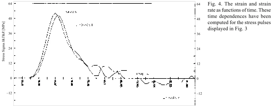
the right interfaces of the specimen, respectively. If we use the obvious assumptions (BUCHAR & BILEK 1984) we may obtain some material characteristics, e.g.: – stress in the specimen σ (t) = σT (t) = σI (t) + σR (t) – strain rate and strain in the specimen:
where:Zb acoustic impedance of the bar
Zb = ρb cb, ρb material density
cb one-dimensional wave velocity
lo specimen length
For our purposes it is convenient to use the frequency domain where the stress pulses are expressed as:
where: S spectral function
The corresponding spectral functions enable to intro-duce the functions describing the transmission and reflec-tion of the stress pulse in the frequency domain as:
[10] dt t I S d t I S t d t I S t d t I S t R T I R T I R I R T T I I ) exp( ) exp( ). ( 1 ) ( ) exp( ). ( 1 ) ( ) exp( ). ( 1 ) ( , , ,
, = σ −ω
ω ω ω π = σ ω ω ω π = σ ω ω ω π = σ
∫
∫
∫
∫
∞ + ∞ − ∞ + ∞ − ∞ + ∞ − +∞ ∞ − ) ( ) ( ) ( , ) ( ) ( ) ( ω ω = ω ω ω = ω I R I T S S R S S T( )
( )
( )
( )
o b T R I l Z t t tt ó ó
å = −σ −
( )t t
MATERIAL AND PROCEDURE
Edam cheese of different age (1–59 weeks) was analy-sed. Samples were prepared from commercially manu-factured Edam bricks; with 30% and 45% fat in dry matter (FDM). A dairy plant processes about 50 000 l of milk a day in a standard manufacturing schedule. Ap-proximately ten sets of 210 Edam bricks (in each batch) are produced. Immediately after salting, 6 bricks (ran-domly chosen) from different batches were cut to 5 slic-es (each about 0.5 kg) and vacuum-packaged in cryovac foil. Samples were stored at 10°C for measurements af-ter given periods. From the block of cheese the speci-mens of 14 mm in diameter and 7 mm in thickness were prepared. These specimens were tested using the meth-od shown in Fig. 2. The test bars are made of PMMA. The acoustic impedance of PMMA is 3.18 MPas/m. The loading stress pulses were initiated by the impact of a short PMMA bar (20 mm in length). An example of the
Fig. 4. The strain and strain rate as functions of time. These time dependences have been computed for the stress pulses displayed in Fig. 3
Fig. 5. Experimental values of the amplitude of the transmission function T. The data have been obtained from the stress pulses reported in Fig. 3
64
48
36
24
12
0
12 64
48
36
24
12
0
12
Stress
Sigma
I
&
T
&
R
[MPa]
Amplitude
of
the
transmission
function
T
Frequency [1/s]
experimental record of the stress pulses σI (t), σT (t) and
σR (t) is given in Fig. 3.
[image:4.595.68.539.97.282.2]The corresponding strain and strain rate are shown in Fig. 4.
These time dependences were computed for the stress pulses displayed in Fig. 3.
These pulses, namely σI (t) and σT (t) were expressed in form of Fourier integral. In this way the function T(ω) which characterises the transmission of the stress pulse through the specimen was obtained. This function is com-plex, i.e.
[14]
An example of the frequency dependence of the ampli-tude of the transmission function T is shown in Fig. 5.
Now we can use the theoretical value of T and by a comparison with the experimental values one can obtain
) (
) * ( exp ) ( * ) ( (
2 2 2
2 2 1
2 1
T T arctg T
T T
I T T I T T
= ϕ +
=
ϕ =
ω + ω = ω
103 104 105 106
the value of α(ω) and c(ω). The procedure is very com-plicated and it is convenient to use the MAPLE software or any similar program. In this way we obtain the left sides of Equations [5]. These are two equations for three un-known parameters E1, E2 and θ. It means we need another equation. We can use Equation [7] which describes the value of c for the infinite frequency. These three equa-tions, i.e. [5] and [7], enable to obtain the parameters of the rheological model which is shown in Fig. 1. These equations are highly nonlinear and the use of the software mentioned above is very convenient. This procedure was applied to the experimental results obtained for the spec-imens of the Edam cheese. For every stage of cheese rip-ening these parameters were determined for three different incident stress pulses (different velocities of the impact of the striker – see Fig. 2). The resulting value of the rheo-logical parameter represents an average of these values.
RESULTS AND DISCUSSION
The parameters of the rheological model shown in Fig. 1 are given in Table 1.
In the given table the values of stress wave propagation at infinite frequency – see Eq. [7] – are also given togeth-er with the values of viscosity (Fig. 1). The quantities given in Table 1 decrease with the time of cheese ripening. This tendency is manifested in Figs. 6–9.
Time of the Cheese Ripening: The obtained results enable to evaluate the dependence of damping and phase velocity on the frequency. The phase velocity c(ω) and damping α(ω) increase with the frequency up to some limit value given by Eqs. [7] and [8]. The phase velocity
c(ω) decreases with the time of cheese ripening (Fig. 9). The damping coefficient at infinite frequency increases with the frequency as shown in Fig. 10.
Fig. 6. The effect of the time of cheese ripening on the elastic moduli
Fig. 7. The effect of the time of cheese ripening on the relaxa-tion time
Fig. 8. The effect of the time of cheese ripening on viscosity
Fig. 9. The effect of the time of cheese ripening on the veloci-ties of the high frequency waves
Time of ripening [weeks]
0 10 20 30 40 50 60
20 40 60 80 100 120 140 160 180 200
Time of ripening [weeks]
Relaxation
time
[µs]
0 10 20 30 40 50 60
0 10 20 30 40 50 60 70 80 90
V
iscotity
[kPas]
Time of ripening [weeks]
0 10 20 30 40 50 60
550 600 650 700 750 800 850 900
Time of ripening [weeks]
Velocity
at
infinite
frequency
[m/s]
Elastic
moduli
[MPa]
0 50 100 150 200 250 300 350 400 450
0 10 20 30 40 50 60
E1
E2 E1
Table 1. The parameters of the Edam cheese rheological model
Time of ripening Density E1 E2 θ c∞ η
[weeks] [kg/m3] [MPa] [MPa] [µs] [m/s] [kPas]
1 1070 380 420 195 873 81.9
2 1080 380 400 190 850 76.0
3 1050 360 410 182 856 73.8
5 1020 360 400 171 863 68.4
6 1020 350 390 165 852 64.4
12 1000 30 360 140 812 50.4
14 1100 310 360 132 780 47.5
18 1060 280 320 117 752 37.4
33 1070 210 270 76 670 20.5
40 1080 200 240 58 638 13.9
59 1060 140 200 32 566 6.4
It means that the stress pulse is attenuated during its propagation. This attenuation increases with the time of cheese ripening.
R e f e r e n c e s
ACHENBACH J.D. (1973): Waves in Elastic Solids. Amster-dam, North Holl. Publ.
AKI K., RICHARDSON P.G. (1980): Quantitative seismology. San Francisco, W.H. Freemand Co.
BREKHOVSKIH L. (1973): Volny v sloistych sredach. Moskva, Nauka.
BUCHAR J., BÍLEK Z. (1984): Chování kovových materiálù pøi vysokých rychlostech deformace. Praha, Academia NÈSAV.
BUCHAR J. (1996): Experimental and theoretical study of the rheological properties of selected cheeses. In: BLAHOVEC J. (Ed.): Stress Relaxation in Solids of Biological Origin. Prague, Czech Univ. Agric. Press: 7886.
HAMAN J., ZDANOWICZ A. (1968): O potrzebie roszerzania studiów nad reologia materialow w rolnictwie. Rocz. Nauk Rol., 2: 6882.
KFOURY M., MPAGANE M., HARDY J. (1989): Effect of cheese ripening on rheological properties Camembert and Saint-Paulin cheeses. Lait, 69: 137149.
KOLSKY H. (1949): An investigation of the mechanical char-acteristics of materials at very high strain rates. Proc. Phys. Soc., B62: 676688.
KONSTANCE R.P., HOLSINGER V.H. (1993): Development of rheological test methods for cheese. Food Technol., 46: 105109.
LAKES R.S. (1999): Viscoelastic solids. New York, CRC Press. WANG L., LABIBES K., AZARI Z., PLUVINAGE G. (1994): Generalization of split Hopkinson bar technique to use viscoelastic bar. Int. J. Impact Engng, 15: 669686.
Received for publication April 20, 2000 Accepted for publication January 18, 2001 The increase is remarkable namely for a time higher
than about 18 weeks. The knowledge of this coefficient is very useful for the description of stress pulse propagation in the viscoelastic body. Let us take a block of viscoelas-tic body which is impacted by a projectile moving with some velocity. If we use a very simple description of this process, the dependence of the stress in the block on the distance x, in the direction of the wave propagation is given by the equation (e.g. WANG et al. 1994):
where: α given by the Eq. [8]
) ( exp )
1 ( 2 exp )
(
2
2 1
x x
E E c
x o = −α
+ η
ρ − σ =
σ ∞
Fig. 10. The frequency dependence of the limit value of damp-ing coefficient (see Eq. 8)
Time of ripening [weeks]
Limit
value
of
damping
[1/m]
0 1 2 3 4 5 6 7 8 9
Corresponding author:
Prof. Ing. JAROSLAV BUCHAR, DrSc., Mendelova zemìdìlská a lesnická univerzita v Brnì, Ústav fyziky, Zemìdìlská 1, 613 00 Brno, tel.: + 420 5 45 13 31 93, fax: + 420 5 45 21 20 44, e-mail: [email protected]
Souhrn
BUCHAR J., KUBI I., GAJDÙEK S., KØIVÁNEK I. (2001): Vliv zrání sýra na vazkopruné vlastnosti eidamského sýra. Czech J. Food Sci., 19: 17.
Byl sledován vliv doby zrání na parametry reologického modelu eidamského sýra. Vzorky sýra byly zatìovány metodou Hopkinsonovy mìrné dìlené tyèe. Byla navrena pùvodní metoda hodnocení výsledkù tohoto zpùsobu zatìování, která umoòuje sledovat vazkopruné vlastnosti. Ukazuje se, e tyto vlastnosti jsou popsány v rámci tzv. standardního modelu lineárního tìlesa. Je vyhodnocen vliv doby zrání na parametry tohoto modelu.