Modelling to Generate Alternatives Using Simulation Driven Optimization: An Application to Waste Management Facility Expansion Planning

(1)

Modelling to Generate Alternatives Using

Simulation-Driven Optimization: An Application to Waste

Management Facility Expansion Planning

Julian Scott Yeomans, Raha Imanirad

OMIS Area, Schulich School of Business, York University, Toronto, Canada Email: syeomans@schulich.yorku.ca, rimanirad09@schulich.yorku.ca

Received May 24, 2012; revised July 3, 2012; accepted July 10, 2012

ABSTRACT

Public sector decision-making typically involves complex problems that are riddled with competing performance ob- jecttives and possess design requirements which are difficult to capture at the time that supporting decision models are constructed. Environmental policy formulation can prove additionally complicated because the various system components often contain considerable stochastic uncertainty and frequently numerous stakeholders exist that hold completely incompatible perspectives. Consequently, there are invariably unmodelled performance design issues, not apparent at the time of the problem formulation, which can greatly impact the acceptability of any proposed solutions. While a mathematically optimal solution might provide the best solution to a modelled problem, normally this will not be the best solution to the underlying real problem. Therefore, in public environmental policy formulation, it is generally preferable to be able to create several quantifiably good alternatives that provide very different approaches and perspectives to the problem. This study shows how a computationally efficient simulation-driven optimization approach that combines evolutionary optimization with simulation can be used to generate multiple policy alternatives that satisfy required system criteria and are maximally different in decision space. The efficacy of this modelling-to-generate-alternatives method is specifically demonstrated on a municipal solid waste management facility expansion case.

Keywords: Simulation-Driven Optimization; Modelling-to-Generate-Alternatives; Environmental Decision Making

under Uncertainty

1. Introduction

Public sector decision-making typically involves complex problems that are riddled with competing performance objectives and possessing performance design requirements which are very difficult to capture at the time that any supporting decision models are constructed [1-4]. Environmental policy formulation can prove even more complicated because the various system components often contain considerable degrees of stochastic uncertainty. Consequently, public sector environmental policy formulation proves to be an extremely complicated and challenging task. While mathematically optimal solutions can provide the best results to the modelled problems, they are frequently not the best solutions to the underlying real problems as there are invariably unquantified issues and unmodelled objectives not apparent at the time the models were constructed [1,2,5]. This is a familiar concern in public sector settings where final decisions tend to be shaped not only by quantified objectives, but also by stakeholder preferences and socio-economic/ political objectives that are extremely subjective in na-

ture. It is often not possible to express these subjective considerations clearly and, therefore, impossible to capture them quantitatively in any optimization model. Consequently, from an environmental policy formulation standpoint it is often preferable to be able to generate several alternatives that provide multiple, disparate perspectives to the particular problem [6,7]. Preferably these alternatives should all possess good (i.e. near-optimal)

objective measures with respect to the modelled objective(s), but be fundamentally different from each other in terms of the system structures characterized by their decision variables [4,7].

(2)

with respect to the modelled objectives, yet very differ- ently with respect to the unmodelled issues.

Yeomans et al. [13] showed how to incorporate data

uncertainty directly into environmental planning using an approach referred to as simulation-driven optimization (SDO). SDO is a family of optimization techniques that incorporates inherent system uncertainties expressed as probability distributions into its computational procedure [14]. Linton et al. [15] and Yeomans [7] have shown that

SDO can be considered an effective, though very computationally intensive, MGA technique for environmental policy formulation. However, none of these SDO MGA approaches have been able to provide guarantees to ensure that the created alternatives are sufficiently different in decision variable structure from one another [16].

In this paper, it is shown how to efficiently generate a set of maximally different solution alternatives for public environmental policy planning situations containing considerable stochastic uncertainty by using a version of the EAGA technique of [12] that has been specifically modified for SDO. This stochastic technique employs a spe- cialized scheme within the SDO procedure to produce sets of alternatives, then screens these solutions to select a small number that are simultaneously both good and very different from each other. The approach is very computationally efficient, since it permits the generation of multiple, good-but-very-different solution alternatives in only a single computational run of the SDO algorithm rather than the multiple separate implementations required in earlier MGA procedures. Since this innovative MGA scheme has the effect of essentially inserting additional subpopulations on top of the original population used for SDO function optimization, the best solution found by the MGA procedure within the subpopulation corresponding to this “original” SDO population will be indistinguishable from a problem’s overall optimal solution. Hence, this new SDO MGA algorithm also per- forms well with respect to its role in function optimization. This study illustrates the efficacy of the MGA capabilities of this new SDO procedure to construct very different, good solutions by testing it on a municipal solid waste (MSW) management facility expansion case study taken from [11].

2. Simulation-Optimization for Function

Optimization

Determining optimal solutions to large stochastic problems proves to be very complicated when system uncertainties have to be accounted for and incorporated directly into the solution procedure [14]. When stochastic conditions exist, values for the constraints and objectives can only ever be efficiently estimated by simulation. SDO is a broadly defined family of solution approaches that combines simulation with some type of optimization

method for stochastic optimization [14]. In SDO, all un- known objective functions, constraints, and parameters are replaced by one or more discrete event simulation models in which the decision variables provide the settings under which the simulation is performed. Since all measures of system performance are stochastic, any potential solution, X, needs to be evaluated via simulation.

As simulation is computationally intensive, an optimization component is used to guide the search for solutions through the problem’s feasible region using as few simulation runs as necessary. Evolutionary algorithms are conducive to these extensive searches because the complete set of candidate solutions maintained in their popu- lations permits concurrent searches to be undertaken throughout multiple sections of the feasible region.

Evolutionary SDO consists of two alternating computational phases: 1) an evolutionary module and 2) a simulation module. Evolutionary SDO maintains a set, or “population”, of candidate solutions throughout its execution. The quality or “fitness” of each solution in this population is found by having its performance criterion,

F, evaluated by simulation. After simulating each candi-

date solution, the respective fitness values become inputs to the evolutionary module for the creation of the next generation of solutions. The fitness of each solution within the population is ranked in comparison to every other candidate solution. These ranked fitness measures are the inputs to the evolutionary module where the next solution population is created using the evolutionary algorithm. The driving force underlying evolutionary procedures is that fitter solutions in a current population possess a greater likelihood for survival and progression into the subsequent generations. After generating a new candidate solution set, the evolutionary module returns the new population to the simulation module for com- parative evaluation. This alternating, two-phase search process terminates when an appropriately stable system state has been attained [7]. The optimal solution produced by the procedure is the single best solution found over the course of the entire search.

3. Modelling to Generate Policy Alternatives

with Simulation-Optimization

(3)

sions are constructed based not only upon clearly stated and modelled objectives, but also upon environmental, political and socio-economic goals and stakeholder preferences that are fundamentally subjective [9,10,12,16].

To illustrate the implications of an unmodelled objective on a decision process, assume that the optimal solution for a quantified, single-objective, maximization decision problem is X* with corresponding objective value

Z1*. Now suppose that there exists a second, unmodelled,

maximization objective Z2 that reflects environmen-

tal/political acceptability. Let the solution Xa, belonging

to the noninferior, 2-objective set, represent a potential best compromise solution if both objectives could some- how have been simultaneously evaluated by the deci-

sion-maker. While Xa might be viewed as the best com-

promise solution to the real problem, it would clearly appear inferior to the solution X* in the quantified model

since it must be the case that Z1a ≤ Z1*. This observation

implies that when unmodelled objectives are factored into decision making processes, mathematically inferior solutions for the modelled problem can potentially be optimal for the real problem. Therefore, when unmodelled objectives and unquantified issues exist, different approaches are required in order to not only search the decision space for the noninferior set of solutions, but also to explore the decision space for inferior alternative solutions to the modelled problem.

In the remainder of this section, an MGA procedure that is capable of incorporating uncertainty directly into its generated alternatives via SDO is developed using a modified adaptation of [12]. In order to properly moti- vate this procedure, it is necessary to provide a more formal definition of the goals of an MGA process [5,7,10]. Suppose the optimal solution to an original

mathematical model is X* with objective value Z* =

F(X*). The following model can then be solved to gener-

ate an alternative solution that is maximally different from X*:

*

M ax 



i XiXi (P1)

. . s t XD

 

*

F X Z T

where Δ is a difference function and T is a target

speci-fied in relation to the original optimal function value Z*. T is a user-supplied value that represents what proportion

of the inferior region should be explored for alternative solutions.

A direct, stepwise method to generate alternatives would be to iteratively solve the maximum difference

model using SDO by incrementally updating the target T

whenever a new alternative has been produced. In this manner, the initial problem formulation would be optimized and then supplementary alternatives would be

generated by systematically adjusting target constraints to force the creation of the suboptimal solutions [10]. While a stepwise approach is straightforward, it would require repeated execution of the SDO algorithm, which would be extremely computationally intensive [7]. How- ever, by using the subsequent approach, it becomes possible to implement an MGA procedure using SDO that produces alternatives which are analogous (but not necessarily identical) to those of the stepwise method. This is a more efficient procedure in that it exploits the population-based searches of evolutionary algorithms in order to represent multiple different solution alternatives simultaneously.

The new MGA procedure is based upon the concept of co-evolution and is designed to generate a small number of good but maximally different alternatives. In this algorithm, subpopulations within the evolutionary algorithm’s overall population concurrently evolve toward different alternative solutions. Each desired solution alternative is represented by one subpopulation that un- dergoes the evolutionary search procedure. This search can be structured based upon any standard evolutionary search procedure containing appropriate encodings and operators that best suit the problem being solved. The survival of solutions in each subpopulation depends upon how well the solutions perform with respect to the modelled objective(s) as well as upon how far they are away from the other solutions in the decision space. Thus, the evolution of solutions in each subpopulation is influ- enced by those solutions contained in the other subpopulations, forcing the evolution of each subpopulation to- wards good but distant regions of the decision space. This co-evolutionary concept enables the design of the following explicit algorithm to search for a set of good solutions that are maximally different from each other.

The main steps within the algorithm are as follows: 1). Create an initial population stratified into P + 1

equal-sized subpopulations. P represents the desired

number of alternative solutions to the overall optimal

solution and must be established a priori by the deci-

sion-maker. Sp represents the pth subpopulation set of solutions, p = 0, ···, P and there are K solutions con-

tained within each Sp. S0 is the subpopulation dedicated to the search for the overall optimal solution to the modelled problem. The best solution from S0 will be used to establish the benchmarks for the relaxation constraint.

2). Evaluate each of the solutions in S0 using simula-tion and identify the best solusimula-tion with respect to the modelled objective. In Sp, p = 1, ···, P, evaluate each of the solutions with respect to the modelled objective using the simulation module. Solutions satisfying the target constraint are designated as feasible, while all other solu-tions are designated as infeasible

(4)

preserve the best individual in each subpopulation. In S0, this is the best solution measured with respect to the modelled objective. In all other subpopulations Sp, p = 1, ···, P, the best solution is the feasible solution most

distant (the distance measure is defined in Step 6) in decision space from all of the other subpopulations. If all solutions in Sp are infeasible, then this is the best individual solution with respect to the modelled objective. This step simultaneously selects a set of alternatives that respectively satisfy different values of the target T while

being as far apart as possible (i.e. maximally different in

the sense of P1) from the solutions generated in each of

the other subpopulations. By the co-evolutionary nature of this algorithm, the alternatives are simultaneously

generated in one pass of the procedure rather than the P

implementations suggested by the necessary increments to T in problem [P1].

4). Stop the algorithm if the termination criterion

(such as maximum number of iterations or some appro-priate measure of solution convergence) has been met. Otherwise, proceed to Step 5.

5). Identify the decision space centroid, Cip, for each of the N decision variables Xikp, i = 1, ···, N, in solution k = 1, ···, K, of Sp, Cip 



1 K



*



kXikp. Each centroid

represents the N-dimensional centre of mass for the solutions in each of the respective subpopulations, p. In the

calculation shown, each dimension of each centroid is computed as the average value of that decision variable over all of the values for that variable within the respect- tive subpopulation. Alternatively, the centroid could be calculated as a fitness-weighted average or by some other appropriately defined measure.

6). For each solution k = 1, ···, K, in each Sq, q ≠ 0, calculate Dkq, a distance measure between that solution and all other subpopulations.



Min ; 1, , ,

kq ikp ip

D  X C p  P pq



.

This distance represents the minimum distance between

solution k in subpopulation q and the centroids of all

other subpopulations.

7). Apply a binary tournament to the solutions in each

Sp. For S0, the selection is with respect to the modelled objective. In each Sp, p ≠ 0, the selection is based on the fitness of the solution with respect to the modelled objective(s) as well as its distance from the other sub-popula- tions Dkp. For each Sp, p ≠ 0, 1) when both solutions are feasible with respect to the relaxed constraint, select the one with the better objective, else 2) if the majority of the solutions are feasible, select based upon the distance measure Dkp, otherwise, 3) select based upon the objective function value. The goal of maximal difference is to force solutions from one subpopulation be as far apart as possible in the decision space from the solutions of each of the other subpopulations. This step identifies the spe-

cific solution in each subpopulation which is as distant as possible from the solutions in all of the other subpopulations. In each Sp, apply recombination operators to the solutions selected and return to Step 2.

By adopting this MGA methodology, multiple design options can be created that meet established system criteria, while simultaneously remaining acceptable and im- plementable in practice. These solutions can considered good from two perspectives: 1) based upon the evolving nature of the search process, all surviving solutions will be extremely fit—corresponding to policy solutions that have necessarily achieved near-optimal measures for their objective functions; and, 2) the solutions found will closely satisfy the required system criteria that each policy option must possess, as represented by the constraints stated within the problem. Consequently, the SDO procedure used within this MGA context automatically generates a set of very good policy alternatives and most of these options would never have been constructed by planners during a normal policy setting phase. Further- more, all of these policy solutions will have their inherent planning uncertainty directly integrated into the generation of these alternatives. SDO’s direct integration of uncertainty into the option generation produces major practical benefits in comparison to solutions created by any other deterministic MGA procedure. And since environmental policy formulation problems contain so many uncertain components, reality dictates that they most likely possess more than one acceptable solution.

In effect, the SDO MGA method expands the population size of a “standard” evolutionary algorithm by ap- pending an additional P subpopulations, Sp, p = 1, ···, P, onto the procedure’s original population, S0. It is the processing of these subpopulations in the MGA algorithm which generates the maximally different solution

alternatives, while subpopulation S0, itself, remains

dedicated to determining the problem’s overall optimal solution via the standard evolutionary optimization procedure employed. Hence, irrespective of the operations occurring in subpopulation Sp, p = 1, ···, P, upon termination of the SDO MGA algorithm, the best solution found residing within S0 should be essentially identical (subject to minor stochastical deviations) to that determined by an SDO procedure operating solely in the role of a function optimizer. Furthermore, when contrasted with the intensive computational requirements necessary in SDO’s simulation phases, the storage and processing impacts attributable to the additional steps related to the additional operations in the evolutionary phases would contribute only a negligible increase to the execution time of any standard evolutionary algorithm. Conse- quently, the process outlined in the above algorithm could be used to readily project MGA capabilities onto

(5)

perhaps the most computationally efficient one) with virtually insignificant additional operational requirements.

By using the maximal difference concept, the SDO- based MGA algorithm produces alternatives which possess objective function bounds that are analogous, but not identical, to those of a more straightforward stepwise approach. While each alternative produced by a stepwise procedure is maximally different only from the single, overall optimal solution together with an objective value which is at least x% different from the best objective (i.e.

x = 1%, 2%, etc.), the new procedure generates alterna-

tives that are no more than x% different from the overall

optimal solution but also with each one of these solutions being as simultaneously maximally different as possible from every other generated alternative that is produced in terms of the solution structure of their decision variables according to [P1].

Finally, the SDO MGA algorithm is a much more efficient process than a stepwise approach to [P1] in that it

exploits the population-based searches of evolutionary algorithms by representing the multiple different solution alternatives simultaneously. Namely, while a stepwise

procedure would be required to run n different times in

order to generate its n alternatives, the new algorithm need only be run a single time to produce its set of alternatives—irrespective of the value of n. Hence, it is much

more computationally efficient.

4. Case Study of SDO Used in MGA for

Municipal Solid Waste Management

Planning

The application of the SDO MGA procedure will be illustrated using the municipal waste management facilities expansion case study taken from [11]. While this section briefly outlines the case, more extensive details and descriptions can be found in [7] and [11]. The notation [a, b] is used to indicate that the value of an uncer-

tain parameter is estimated to lie within the interval between the values of a and b. Furthermore, if variable A

represents an uncertain parameter specified by the interval [a, b], then the uncertainty of this variable will be

indicated with the notation A . For consistency, pa-

rameters which are constants can be directly represented using the notation, A, by the interval [a, a].

The region in the facility expansion planning problem contains three separate municipalities whose MSW disposal needs are collectively met by a landfill and two waste-to-energy (WTE) incinerators. The planning horizon consists of three separate time periods with each of the periods covering an interval of five years. At the start of the planning period, the landfill possesses an existing capacity of [0.625, 0.775]  106_{tonnes and WTE facili-}

ties 1 and 2 have processing capacities of [100, 125] and [200, 250] tonnes/day, respectively. Both WTE facilities generate waste residues of approximately 30% of the incoming waste streams on a mass basis, and the revenue from the resulting energy re-sale is approximately [15, 25] $/tonne of combusted material. The landfill capacity can be expanded only once over the entire 15 year planning

horizon by an increment of [1.55, 1.70]  106_tonnes.

Each of the WTE facilities can be expanded by any one of four possible options in each of the three time periods. The maximum possible expansion option in any single time period would increase the processing capacity of a WTE facility by 250 tonnes/day. These expansion costs escalate temporally in order to reflect anticipated future conditions and have been discounted to present value cost terms for use in the objective function. The MSW waste generation rates and the costs for waste transportation and treatment vary both temporally and spatially.

The MSW problem requires the determination of the preferred facility expansion alternatives during the different time periods and the effective allocation of the relevant waste flows in order to minimize the total system costs over the planning horizon. In the mathematical model, the type of waste management facility is identified by subscript i, with i = 1 representing the landfill,

and i = 2 and i = 3 corresponding to WTE facilities 1 and

2, respectively. The three municipalities from which the waste originates will be identified using subscript j, j = 1,

2, 3. Subscript k, k = 1, 2, 3, corresponds to the time pe-

riod and m, m = 1, 2, 3, 4, denotes the expansion option

selected for the WTE facilities. The decision variables for the problem will be designated by xijk, yk and zimk, where xijk represents the proportion of solid waste sent from municipality j to waste processing facility i in pe-

riod k; yk corresponds to a binary decision variable for landfill expansion at the start of time period k (yk = 1 if the landfill expands in period k, 0 otherwise), and zimk represents a binary decision variable corresponding to the particular expansion option, m, selected for WTE facility i, i = 2, 3, at the start of period k.

The total cost of waste management, in $/tonne, for the waste flowing from municipality j to processing facility i

in period k is represented by ijk. The per tonne cost for transporting waste from municipality j to facility i in pe-

riod k is ijk

C

TR , and OP _ik is the per tonne operating cost

of processing facility i in period k. The transportation

cost per tonne of waste from WTE facility i to the landfill

in period k is denoted by FTik



, for i = 2, 3. If FE repre-

sents the residue flow rate from a WTE facility to the landfill, expressed as a percentage of the incoming mass

to the WTE facility, and k denotes the per tonne

revenue from the WTE facilities in period k, then RE

1jk 1jk 1

(6)

and Cijk TRijkOPikFE FT



ikOPik



REk,

     

for i = 2, 3, j = 1, 2, 3, and k = 1, 2, 3. The existing ca-

pacity of the landfill, in tonnes, is LC and k



LC 

represents the additional capacity resulting from the landfill expansion undertaken in period k, k = 1, 2, 3;

where the cost of this landfill expansion is FLCk



. The existing capacity, in tonnes per day, for WTE facility i, i

= 2, 3 is i. The amount of incremental capacity ex-

pansion, in tonnes per day, under option m, m = 1, 2, 3, 4,

for WTE facility i,i = 2, 3, at the start of period k, k = 1,

2, 3, is provided by imk; with imk

TC

TC

 FTC correspond-

ing to the capital cost of this expansion. Finally, if the number of days in time period k is Lk and if the number of tonnes of waste generated daily by municipality j dur-

ing period k is WGjk



, then the complete mathematical model for MSW management expansion planning is to:

3 4 3

1

2 1 1

3 3 3

1 1 1

Minimize

Cost k k k imk imk

i m k

k ijk jk ijk

i j k

FLC y FTC z

L C WG x

         





    (1) Subject to: 3 3 1

1 1 2

1

, 1, 2,3

k

k jk jk jk ijk

j k i

k

k k k

L WG x WG x FE

LC y LC k

       _      





      3 (2) 3 4

1 1 1

, 2,3, 1, 2,3

k

jk ijk imk imk i

j m k

WG x TC z TC i k

           







  (3) 3 1

, 1, 2,3, 1, 2,

jk ijk jk

i

WG x WG k j



  



  (4)

4

1

1, 2,3, 1, 2,3

imk m

z i k



  



(5)

3 1 1 k k y  



(6) 3

1

1, 1, 2,3, 1, 2,3

ijk i

x j k



  



(7)

1xijk 0,i1, 2,3, j1, 2,3,k1, 2,3 (8)

or

0 1, 1, 2,3

k

y  k (9)

or

0 1, 2,3, 1, 2,3, 1, 2,3,4

imk

z  i k m (10)

The objective function (1) contains components relat- ing to the cost/benefit effects resulting from different waste management decisions and the capital costs required for expanding the processing facilities. Con-

straints (2) and (3) ensure that the upper limits for waste treatment and disposal in any time period are determined by both the existing facility capacity and any incremental expansion activities occurring in time period k', k' = 1, 2,

3, for the landfill and WTE facilities. The dynamic aspects of these constraints result from such considerations as future economic development, population increase, and environmental management activities. Constraint (4) establishes the waste disposal quantities generated by each of the three municipalities in each time period. Constraint (5) requires that only one option for each WTE facility expansion can be selected in any given time period, and constraint (6) stipulates that the landfill could be expanded only once over the entire planning time horizon. Constraint (7) ensures the disposal of all waste generated by each municipality in every time period. Finally, constraints (8) to (10) provide the technical rela- tionships for the decision variables.

To complete the formulation, Tables 1 and 2 show the

actual values of the various parameters used within the

model. Table 1 provides the detailed numerical informa-

tion regarding the various capital costs and expansion options for both the landfill and WTE facilities. It should be duly noted that all of the capital costs are expressed in present value dollars. Table 2 gives the details for the

[image:6.595.306.539.478.742.2]

waste generation rates for the three municipalities, the operating costs for the three processing facilities, and the transportation costs for waste flows between municipalities and processing facilities over each of the three time periods.

Table 1. Capacity expansion options and their costs for the landfill and WTE facilities.

Time period k = 1 k = 2 k = 3

Capacity expansion option for WTE facility i, i = 2, 3 (tonnes/day):

1

i k

TC

 (option 1) 100 100 100

2

i k

TC

 (option 2) 150 150 150

3

i k

TC

 (option 3) 200 200 200

4

i k

TC

 (option 4) 250 250 250

Capacity expansion option for the landfill (106_tonnes):

k

LC

 [1.55, 1.70] [1.55, 1.70] [1.55, 1.70] Capital cost of WTE facility expansion, i = 2, 3 ($106 present value):

1

i k

FTC (option 1) 10.5 8.3 6.5

2

i k

FTC (option 2) 15.2 11.9 9.3

3

i k

FTC (option 3) 19.8 15.5 12.2

4

i k

FTC (option 4) 24.4 19.1 15.0

Capital cost of landfill expansion ($106_{present value):}

k

(7)

[image:7.595.57.539.99.485.2]

Table 2. Waste generation, transportation costs, and facility operating costs.

Time period k = 1 k = 2 k = 3

Waste generation (tonnes/day):

1k

WG



(Municipality 1) [200, 250] [225, 275] [250, 300]

2k

WG



(Municipality 2) [375, 425] [425, 475] [475, 525]

3k

WG (Municipality 3) [300, 350] [325, 375] [375, 425]

Cost of waste transportation to the landfill ($/tonne):

11k

TR

 (Municipality 1) [12.1, 16.1] [13.3, 17.7] [14.6, 19.5]

12k

TR

 (Municipality 2) [10.5, 14.0] [11.6, 15.4] [12.8, 16.9]

13k

TR (Municipality 3) [12.7, 17.0] [14.0, 18.7] [15.4, 20.6]

Cost of waste transportation to WTE facility 1 ($/tonne):

21k

TR



(Municipality 1) [9.6, 12.8] [10.6, 14.1] [11.7, 15.5]

22k

TR



(Municipality 2) [10.1, 13.4] [11.1, 14.7] [12.2, 16.2]

23k

TR (Municipality 3) [8.8, 11.7] [9.7, 12.8] [10.6, 14.0]

Cost of waste transportation to WTE facility 2 ($/tonne):

31k

TR

 (Municipality 1) [12.1, 16.1] [13.3, 17.7] [14.6, 19.5]

32k

TR

 (Municipality 2) [12.8, 17.1] [14.1, 18.8] [15.5, 20.7]

33k

TR (Municipality 3) [4.2, 5.6] [4.6, 6.2] [5.1, 6.8]

Cost of residue transportation from the WTE facilities to the landfill ($/tonne):

2k

FT (WTE facility 1) [4.7, 6.3] [5.2, 6.9] [5.7, 7.6] 3k

FT (WTE facility 2) [13.4, 17.9] [14.7, 19.7] [16.2, 21.7] Operational cost ($/tonne):

1k

OP (Landfill) [30, 45] [40, 60] [50, 80]

2k

OP

 (WTE facility 1) [55, 75] [60, 85] [65, 95]

3k

OP (WTE facility 2) [50, 70] [60, 80] [65, 85]

Using this model, Yeomans [7] solved this problem using SDO strictly as a function optimizer and produced a single best solution to the expansion problem costing $600.2 million. As outlined earlier, when public policy planners are faced with difficult and potentially contro- versial choices, they generally prefer to be able to select from a set of near-optimal alternatives that differ signify- cantly from each other in terms of the system structures characterized by their decision variables. In order to create these alternative planning options, it would be possible to place extra target constraints into the original

model as in [P1] which would force the generation of

solutions that were different from this newly determined, optimal solution. By including such a technical constraint on the objective function, Yeomans [7] created three alternative expansion options that increased the total system cost of the original, optimized model by target values of 2%, 5%, and 8%, respectively. By adding these specific constraints to the original model, the problem needed to be resolved an additional three times.

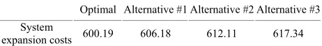
However, to improve upon the process of running four separate instances of the SDO algorithm to determine these solutions, the co-evolution aspects of the MGA procedure described in the previous section was run only once, thereby directly producing the 4 alternatives shown in Table 3. The evolutionary parameters used in this

computational experiment were a population size of 100, a maximum number of iterations of 300 (together with an additional check for solution convergence), a crossover parameter of 40% and a mutation rate of 5%.

(8)

[image:8.595.57.288.114.147.2]

Table 3. System expansion costs ($ millions) for the 4 maxi-mally different alternatives.

Optimal Alternative #1 Alternative #2 Alternative #3 System

expansion costs 600.19 606.18 612.11 617.34

performance with respect to the unmodelled issues, thereby incorporating the unmodelled issues into the actual solution process. This example has demonstrated how the SDO MGA modelling approach can be used to efficiently generate multiple, good policy alternatives that satisfy required system performance criteria according to prespecified bounds within highly uncertain envi- ronments and yet remain as maximally different from each other as possible in the decision space.

Given the performance bounds established for the objective in each problem instance, the decision-makers can feel reassured by the stated performance for each of these options while also being aware that the perspectives provided by the set of dissimilar decision variable structures are as maximally different from each other as is feasibly possible. Hence, if there are stakeholders with income- patible standpoints holding diametrically opposing view- points, the policy-makers can perform an assessment of these different options without being myopically con- strained by a single overriding perspective based solely upon the objective value. In addition to its alternative generating capabilities, the SDO MGA procedure has simultaneously performed exceedingly well with respect to its role in function optimization. Although a mathematically optimal solution may not provide the best approach to the real problem, it can be demonstrated that the MGA procedure has indeed produced a very good solution value for the originally modelled optimization problem, itself. It should be explicitly noted that the cost of the overall best solution produced by the MGA procedure (i.e. the solution S0) is indistinguishable from the one determined in the function optimization process of [7].

In totality, the results of this section underscore several important findings with respect to the use of SDO within this MGA procedure: 1) SDO can be used to generate more good alternatives than planners would be able to create using other MGA approaches because of the evolving nature of its population-based solution searches; 2) All of the solutions produced by SDO incorporate system uncertainties directly into their structure during their creation unlike all of the earlier deterministic MGA methods; 3) The alternatives generated are good for planning purposes since their structures are all as maximally different from one another as possible (i.e. these

differences are not just simply from the overall optimal solution); 4) The MGA procedure is computationally very efficient since it need only be run once to generate

its entire set of multiple, good solution alternatives (i.e.

to generate n solution alternatives, MGA needs to run

exactly the same number of times that SDO would need to be run for function optimization purposes alone, ire- spective of the value of n); and, 5) The best overall solu-

tions produced by the MGA procedure will be very simi- lar, if not identical, to the best overall solutions that would be produced by SDO for function optimization alone.

5. Conclusions

Public environmental policy formulation is a very complicated process that can be impacted by many uncertain factors, unquantified issues and unmodelled objectives. This combination of uncertainties and unknowns together with the competing interests of various stakeholders ob- ligates public policy-makers to integrate many conflict- ing sources of input into their decision process prior to final policy adoption. In this paper, a computational procedure was presented that showed how SDO could be used to efficiently generate multiple, maximally different, near-best policy alternatives for difficult, stochastic, environmental problems and the effectiveness of this MGA approach was illustrated using a case study of municipal solid waste facility expansion planning.

In this stochastic MGA capacity, SDO was shown to efficiently produce numerous solutions possessing the requisite characteristics of the system, with each generated alternative providing a very different planning perspective. Because an evolutionary method guides the search, SDO actually provides a formalized, population-based mechanism for considering many more solution options than would be created by other MGA approaches. However, unlike the deterministic MGA methods, SDO incorporates system uncertainties directly into the generation of these alternatives. MSW systems provide an ideal testing environment for illustrating the wide variety of modelling techniques used to support public policy formulation, since they possess all of the prevalent incongruencies and system uncertainties that so often exist in complex planning processes. Since SDO techniques can be adapted to model a wide variety of problem types in which system components are stochastic, the practicality of this co-evolutionary MGA approach can clearly be extended into numerous disparate operational and strategic planning applications containing significant sources of uncertainty.

REFERENCES

(9)

doi:10.1007/s11269-006-9099-y

[2] J. A. E. B. Janssen, M. S. Krol, R. M. J. Schielen and A. Y. Hoekstra, “The Effect of Modelling Quantified Expert Knowledge and Uncertainty Information on Model Based Decision Making,” Environmental Science and Policy, Vol.13, No. 3, 2010, pp. 229-238.

doi:10.1016/j.envsci.2010.03.003

[3] H. T. Mowrer, “Uncertainty in Natural Resource Decision Support Systems: Sources, Interpretation and Impor- tance,” Computers and Electronics in Agriculture, Vol. 27, No. 1-3, 2000, pp. 139-154.

doi:10.1016/S0168-1699(00)00113-7

[4] W. E. Walker, P. Harremoes, J. Rotmans, J. P. Van der Sluis, M. B. A. Van Asselt, P. Janssen and M. P. Krayer von Krauss, “Defining Uncertainty—A Conceptual Basis for Uncertainty Management in Model-Based Decision Support,” Integrated Assessment, Vol. 4, No. 1, 2003, pp. 5-17. doi:10.1076/iaij.4.1.5.16466

[5] D. H. Loughlin, S. R. Ranjithan, E. D. Brill and J. W. Baugh, “Genetic Algorithm Approaches for Addressing Unmodeled Objectives in Optimization Problems,” Engi- neering Optimization, Vol. 33, No. 5, 2001, pp. 549-569. doi:10.1080/03052150108940933

[6] M. Matthies, C. Giupponi and B. Ostendorf. “Environ- mental Decision Support Systems: Current Issues, Meth-ods and Tools,” Environmental Modelling and Software, Vol. 22, No. 2, 2007, pp. 123-127.

doi:10.1016/j.envsoft.2005.09.005

[7] J. S. Yeomans, “Applications of Simulation-Optimization Methods in Environmental Policy Planning UNDER Un- certainty,” Journal of Environmental Informatics, Vol. 12, No. 2, 2008, pp. 174-186. doi:10.3808/jei.200800135 [8] B. W. Baetz, E. I. Pas and A. W. Neebe, “Generating

Alternative Solutions for Dynamic Programming-Based Planning Problems,” Socio-Economic Planning Sciences, Vol. 24, No. 1, 1990, pp. 27-34.

doi:10.1016/0038-0121(90)90025-3

[9] J. W. Baugh, S. C. Caldwell and E. D. Brill, “A Mathe-

matical Programming Approach for Generating Alterna- tives in Discrete Structural Optimization,” Engineering Optimization, Vol. 28, No. 1, 1997, pp. 1-31.

doi:10.1080/03052159708941125

[10] E. D. Brill, S. Y. Chang and L. D. Hopkins, “Modelling to Generate Alternatives: The HSJ Approach and an Il- lustration Using a Problem in Land Use Planning,” Man- agement Science, Vol. 27, No. 3, 1981, pp. 314-325. doi:10.1287/mnsc.28.3.221

[11] J. S. Yeomans and Y. Gunalay, “Simulation-Optimization Techniques for Modelling to Generate Alternatives in Waste Management Planning,” Journal of Applied Op- erational Research, Vol. 3, No. 1, 2011, pp. 23-35. [12] E. M. Zechman and S. R. Ranjithan, “An Evolutionary

Algorithm to Generate Alternatives (EAGA) for Engi- neering Optimization Problems,” Engineering Optimiza- tion, Vol. 36, No. 5, 2004, pp. 539-553.

doi:10.1080/03052150410001704863

[13] J. S. Yeomans, G. H. Huang and R. Yoogalingam, “Com- bining Simulation with Evolutionary Algorithms for Op- timal Planning Under Uncertainty: An Application to Municipal Solid Waste Management Planning in the Re- gional Municipality of Hamilton-Wentworth,” Journal of Environmental Informatics, Vol. 2, No. 1, 2003, pp. 11- 30. doi:10.3808/jei.200300014

[14] M. C. Fu, “Optimization via Simulation: A Review,” Annals of Operational Research, Vol. 53, No. 3, 2002, pp. 199-248. doi:10.1287/ijoc.14.3.192.113

[15] J. D. Linton, J. S. Yeomans and R. Yoogalingam, “Policy Planning Using Genetic Algorithms Combined with Simulation: The Case of Municipal Solid Waste,” Envi- ronment and Planning B: Planning and Design, Vol. 29, No. 5, 2002, pp. 757-778. doi:10.1068/b12862