Estimation methods for regression models with unequal error variances

warwick.ac.uk/lib-publications

A Thesis Submitted for the Degree of PhD at the University of Warwick

Permanent WRAP URL:

http://wrap.warwick.ac.uk/94472

Copyright and reuse:

This thesis is made available online and is protected by original copyright. Please scroll down to view the document itself.

Please refer to the repository record for this item for information to help you to cite it. Our policy information is available from the repository home page.

WITH UNEQUAL ERROR VARIANCES

GHULAM RASUL PASHA

THESIS SUBMITTED IN FULFILLMENT OF THE REQUIREMENTS

FOR THE DEGREE OF DOCTOR OF PHILOSOPHY

UNlVERS ITY OF WARWICK

DEPARTMENT OF STATISTICS

CHAPTER 1 2 3 4 5

TABLE OF CONTENTS

INTRODUCTION AND REVIEW OF EXISTING TECHNIQUES •••••••••••

1.1 1.2 1.3 1.4 1.5 1.6 1.7

Introduction ... .

The MINQUE Principle •••••••••••••••••••••••••••••••• Maximum Likelihood Estimation •••••••••••••••••••••••

Least Square Method •••••••••••••••••••.••••.•.••••••

Weighted Least Square Method ••••••••••••••••••••••••

Purpose of the Thesis ••••••••••••.••.••••••••.••••.• Outline of the Thesis •••••••.•..••••••.•••••••••••••

LARGE SAMPLE PROPERTIES OF WLS AND MINQU-BASED ESTnIATOrrS

2.1 2.2 2.3 2.4 2.5

Introduction . . . • . . . • . . . • • . . .

Asymptotic Results ••••••••••••••••••••.•••.•••••••••

Proof of Theorems ...•••..•.•... ~ ...•..

Non-Normal Case •••••••••••••••••••• e • • • • • • • • • • • • • • • • •

Special Cases of the Theorems •••••••••••••••••••••••

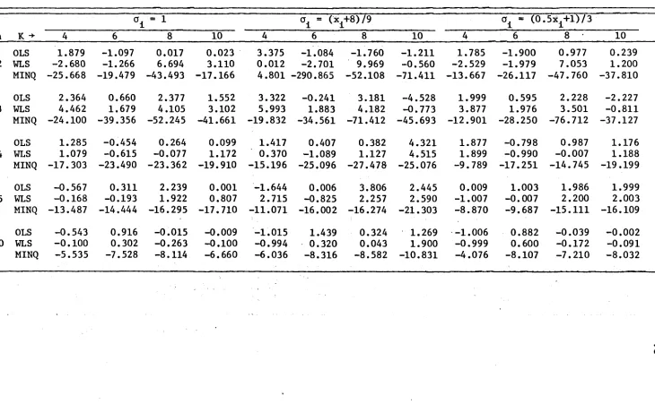
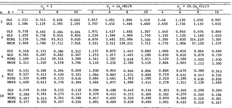
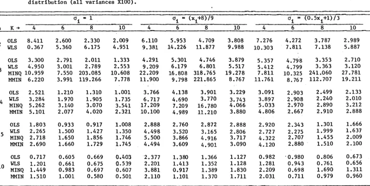
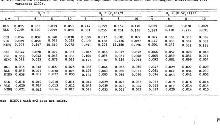
AN EMPIRICAL STUDY OF WLS AND MINQ-BASED ESTIMATORS FOR SMALL SA}1EtLE S. • • • • • • • • • • • • • • • • • • • • • • • • • • • • • • • • • • • • • • • • • • •

3.1 3.2 3.3 3.4

Introduction •••••••••••••••••••••••••••••••••••••••• Sampling Experiments and Computations •••••••••••••••

Empirical Results ... .

Results and Discussion ••••••••••••••••••••••••••••••

USE OF POSTERIOR LIKELIHOOD IN ESTIMATION ••••••••••••••••

4.1 4.2

4.3

4.4

Introduction ... .

Posterior Likelihood Estimators for the Regression

Model ••••••••••••••••••••••••••••••••••••••••.••••••

Empirical Results and Procedures ••••••••••••••••••••

Res ul ts an d Dis cussion ...•.•..• 0 • • • • • • •

ADAPTIVE PROCEDURES IN ESTIMATION OF REGRESSION PARAMETERS

5.1 5.2 5.3

Introduction ... : ... .

Tests of Variance Equality •••••••••••••••••••••••••• Adaptive Procedures for Estimation •• : •••••••••••••••

6 USE OF ADAPTIVE PROCEDURES IN THE ESTIMATION OF REGRESSION PARAMETERS BY GROUPING COMMON VARIANCES... 132

7

8

6.1 Introduction... 132

6.2 Multiple Comparison Methods... 132 6.3 A Multiple Comparisons Test for the Error Variances. 134

6.4 Conclusion 136

ESTIMATION FOR THE ERRORS-IN-VARIABLES MODEL ••••••••••••• 140

7.1 Introduction... 140

. 7.2 Maximum Likelihood Estimators (Equal Variances C~~a) 141 7.3 Maximum Likelihood Estimators (Different Variances

Case) . • . • . • • . • . • • • . . • • • • • • . . • . . • • • • . • • • • • • . • • . • . . • • . 144

7.4 Large Sample Properties of ML (Common Variance Case) 146 7.5 Large Sample Properties of ML (Unequal Variances

Case) • • • • . • . . • . • • . . . • . . . . • . • . • • • • . • . • • • . . . 148

7.6 Method of Least Squares... 150 7.7 Empirical Results... 152

CONCLUSIONS ••••••••••••••••• e.a • • • • • • • • • • • • • • • • • • • • • • • • • • • 155

ACKNOWLEDGEMENTS

As is true of any such intellectual effort. the fundamental

pre-requisite for success is a mentor who embellishes the intellectual

strengths and moral fibre of a student. Professor Keith Ord is a

prototype of an ideal mentor. His brilliance is only matched by his

tolerance for my shortcomings. I would like to thank him especially.

Thanks are also due to Professor P. J. Harrison. Chairman. Department

of Statistics. Warwick University. and Professor George Heitman. Chairman.

Division"of Management Science, The Pennsylvania State University, USA,

for their support and encouragement. I would also like to thank the

Centre for Research, College of Business Administration, The Pennsylvania

State University, for providing the computer time and Mrs. Bonnie K.

Henninger for typing.

I would like to thank my wife. who has endured my whimsical moods

and prolonged separation without the slightest hint of a complaint.

Finally. I would like to humbly dedicate this dissertation to my

supervisor. Professor Keith Ord. a helpful and patient mentor and to my

mother whose love and affection gave me ·the emotional strength to

In this dissertation, we consider estimation procedures for the linear model when the observations are replicated but the error variances are unequal.

The aim of this research was to consider several standard methods for parameter estimation, namely Ordinary Least Squares, Weighted Least Squares, and Maximum Likelihood and to compare these with newly developed procedures. These new techniques included the use of a prior likelihood function to induce "shrinkage" towards a common value among the estimators for the error variances and procedures based on preliminary tests of the hypothesis of variance equality. Both an overall test of equality and a multiple comparison method were considered. In addition, variance

estimates based on MINQUE (Minimum Norm Quadratic Unbiased Estimator) were investigated. The MINQU estimators tend to "stretch out" the variances and were found to be unsatisfactory.

The performance of the above-mentioned approaches was investigated both through asymptotic theoretical results and small samples simulation studies. The results from these two approaches were found to be in broad agreement.

Overall, the multiple comparison and prior likelihood procedures appear to perform best, but the prior likelihood depends upon the avail-ability of satisfactory prior information. So the multiple comparison procedure appears to be the most effective technique in general.

A further study was also conducted to examine the effects of "errors-in-variables." In general it is found that maximum likelihood is

CHAPTER 1

INTRODUCTION AND REVIEW OF EXISTING TECHNIQUES

1.1 Introduction

In the usual analysis of variance m~del, a typical observation is

considered to be the result of some fixed effects and an error term

combined in a linear fashion. In such models, interest mainly lies in

estimating linear functions of the effects. There are, however,

situations whe~e in addition to estimating the linear functions of

effects, the main interest is also concerned with the estimation of the

variances of the effects. Effects of this nature are called random effects

and variances associated with them are called variance components. A

linear model in its generality may, of course, include some fixed and

some random effects. Such a model is referred to as a variance

components model. A linear regression model with a diagonal covariance

matrix is a special case of the variance components model. In such a

model, estimation of the unequal variances is our main goal as a way

to generate improved estimators for the parameters describing the

effects.

There is a vast literature on the topic of estimation of variance

components. The usual mixed linear model discussed in the literature

on variance components is

(1.1.1)

\ is a fixed unknown p-vector of parameters, u

i is a given (nXni) matrix

and ~i is an ni-vector such that

(1.1.2)

2 The Unknown parameterso

i, i-1,2, ••• ,k are called variance components.

A systematic study of the estimation of variance components was

undertaken by Henderson (1953) who proposed three methods of estimation.

But some of the early users of such models are due to Cochran (1939),

Yates and Zacopancy (1935), Fairfield Smith (1936), Yates (1940), Panse

(1946), Rao (1947, 1953, 1956), Henderson (1950) and Brown1ee (1953)

in different fields of applications.

The general approach in all. these papers was to obtain k'

quadratic functions of !., say Y'A

i!., i-1,2, ••• ,1<:'--: which are invariant

for translation of Y by Xa where a is arbitrary, and solve the

equatiqns.'

(1.1.3)

The method of choosing the quadratic forms was intuitive in nature

(see Henderson, 1953) and did not depend on any stated criteria of

estimation. The entries in the ANOVA table giving the sumS of squares

due to different effects were considered as good choices of the

quadratic forms in general. The ANOVA technique provides good

esti-mators in what are called balanced designs (see Anderson, 1975;

Anderson and Crump, 1967) but, as shown by See1y (1975), such estimators

may be inefficient in more general linear models •. For a general

simplicity) and limitations (lack of uniqueness, inapplicability and

inefficiency in special cases), see the papers by Searle (1968, 1971),

See1y (1975), 01sen et al. (1976), and Harvi11e (1977).

Hart1ey and Rao (1967) initiated a different approach in the

maximum likelihood (ML) method. They· considered the likelihood of the

2

unknown parameters~, cri' i-1,2, ••• ,k~~ based on observed Y and obtained

the likelihood equations by computing the derivatives of the likelihood

w.r. to the parameters. Patterson and Thompson (1975) considered

another approach the marginal likelihood or the maximal invariant of

J. .

Y,

e'Y

e -

what are called marginal maximum likelihood (MML) equations. Harvi11e

(1977) has reviewed the ML and MML meth~ds and the computational algorithms

associated with them.

Maximum likelihood estimators, though consistent,may be heavily

biased in small samples so that some caution is needed when they are

used as estimates of individual parameters. The problem is not acute if

the exact distribution of the ML estimator is known, since in that case,

appropriate bias adjustments can be made in the individual estimators

before using them. The general large sample properties associated with

ML estimators are misleading in the absence of studies on the orders of

sample sizes for which these properties hold in particular cases. The

bias in the MML estimators may be slight even in small samples. As

observed earlier, the MML estimator is, by construction, a function of

e'y

estimator is a function of

e'y

There are important practical cases where reduction of Y to

e'y

in the non-identifiability of individual parameters, in which case,

C. R. Rao (1970, 1971a, 1971b, 1972, 1973) proposed a new principle

of estimating heteroscedastic variances and covariances components

called MINQUE (minimum norm quadratic unbiased estimation, estimator

or estimate, depending on context) the scope of which has been extended

to cover a variety of situations by Focke and Dewess (1972), Kleffe

(1975, 1976, 1977a, 1977b, 1978, 1979), J. N. K. Rao (1973), Fuller and

J. N. K. Rao (1978), P. S. R. S. Rao and Chaubey (1978), P. S. R. S.

Rao (1977), Puke1sheim (1977, 1978a), Sinha and Wieand (1977), and

RaO (1979).

1.2 The MINQUE Principle

Consider the variance component model

Y - X@.. + u ~ + ••• +u. ~

- 1-1 K-k (1.2.l)

where Y is an n-vector of observations, X is an (nxp) known matrix,

a

is a p-vector of parameters, u

i is a given (nxni) matrix and ~i is an ni-vector such that

We can express the above model in a compact form

Y - X~

+

where

u"

f' -

From (1.2.2) we have

E(Y) - X~

(1.2.3)

c.

2 2 2

a

P1or+ ••• +Pkok of the variance components 0l, ••• ,ok by a quadratic

function y' AY of random variab1es· .. Y. He developed the following criteria

for determining the matrix A.

1.2.1 Invariance Under Translation of the SParameters. Instead

of

B,

B-BO

BO

Model (1.2.3) becomes

Y - XB - Xy+Ut;

- -0 _

in which case the estimator of t

Pi~

(1.2.5)

(1.2.6)

But (1.2.6) should have the same numerical value as Y'AY whatever

BO

may be. Thus, we require that

- Y'AY + 28 'X'AY + _~

B

- . ~ -0 (1. 2.7)

The above equation is satisfied if

AX -

o.

1.2.2 Unbiasedness. With restriction (1.2.8)

y'AY - ~'X'AX~+ 2~'X'AUt; + t;'U'AUt;

- -

-which reduces to

2 2

For Y'AY to be unbiased for rpiOi for all ai' we require

i

since

E(Y'Ay)

=

E(~'U'AU~)

=

i

k

E(~'U'AU ~) -

r

(1.2.10)

k 2

- r

i-1

.

Here tr stands for trace and vi - ui'u

i • Equation (1.2.10) becomes

which implies that

i-1,2, ••• , k .

1.2.3 Minimum Norm. If the hypothetical variables

2

a natural unbiased estimator of L PiO

i would be

i

(1.2.13)

~ were known,

But the proposed estimator is ~'U'AU~. Hence we would like to

choose A such that the difference ~'(U'AU-~)~ is minimized. Since ~ is

unknown, Rao suggests that A is chosen to minimize

Ilu'

,

where

11-11

Euc1idean norm, the matrix A of the quadratic form Y'AY should be

determined by minimizing

(1. 2.15)

subject to (1.2.8) and (1.2.13). Under the condition ·in (1.2.13)

Pi tr U'AU~ - t~AU~U' - tr AL - - u u '

i ni i i

and hence

tr(U'AU-~)2

U'AU~

~2

- tr U'AUU'AU _ tr

~2

2

- tr AVAV - tr ~

(1.2.16)

2

Thus minimizing tr(U'AU-6) , Subject

2 to (1.2.8) and (1.2.13) is equivalent to minimizing tr AVAV - tr 6 or

equivalently minimizing tr AVAV, since ~ is given, subject to (1.2.8)

and (1.2.13). Thus, the principle of estimation may be described as

follows.

The quadratic form Y'AY is said to be the MINQUE (Minimum Norm

2

Quadratic Unbiased Estimator) of L Piai where the matrix A is determined

i

such that tr AVAV is minimized subject to the conditions (1.2.8) and

(1. 2.13).

c.

invariance which may be stated as follows. The quadratic form Y'AY is

2

said to be the MINQUE without invariance of L Piai if the matrix A is 1

determined such that tr A(V + 1 XX')A(V + 1 XX') is minimized subject

2 2

to the conditions

X'AX -

1.2.4 Examples of MINQUE. C. R. Rao (1970) derives the MINQUE

explicitly for some cases.

(i) When E(Y) -

X~

Gauss-Markov estimator.

(1i)

coincides with the estimator of Anscombe and Tukey (1963).

(iii) _{When E(Yi) - ~ and V(E} 2

i) -

ai'

2 s

2 where Y - (Lyifn) and (n-l)s

Note: An intuitively appealing but biased set of estimators for this'

-2 n - 2

problem would be a i - (n-l) (Yi-Y) ; (1.2.20)

By contrast with MINQUE which "stretches out" the estimators,

(1.2.20) provides an element of "shrinkage" towards the overall mean -2 1 2

a - n La_{i .}

(iv) For the one-way random effects model with E(y

ij) -1Jand V(Yij)

-a~

+

~.

for a2 and a2 are the same as the usual ANOVA estimators.

Cl

(v) Now consider the multivariate model

i-I,2, ••• ,p (1. 2. 21)

where Y

i is an n vector, Xi is a known (nxmi) matrix,

a

vector and Ei is an n-vector with mean zero and E(EiE

j ') - oijI. For the restricted form the model is written as

Y -

xa

+

i

where y' - (Y_l'IY₂

'1 •••

E' -

IEp~)'

a

diagonal matrices with elements Xi and

a

i respectively. Writing D(~

in the form of (L:2.4), we obtain the MINQUE of 0ij as

a

ij - ei ej ftr QiQj

where Q - I - X (X 'X )~ X '

i i i i i~ Ze11ner and Huang (1962)

obtained this estimator for p-2 through a different approach. For the

Y

=

where ® denotes the Kronecker product of two matrices; and Y and E are

as above, but X - (X1Ix21 ••• Ix ) and e' - (el' Isi'I ••• le '). The MINQUE

p . p

can now be shown to be 0ij - ei'ej/tr Q where Q - I - X(X'X)-X' and

e

i

=

(1962).

1.2.5 PropertiesofMINQUE. (i) Additivity: If SI and S2 are the

MINQUE of Pl'a and P2'a respectively, then (Sl+S2) is the MINQUE of

(Pl+P2)

'a.

(ii) Invariance: Consider a non-singular transformation Z - BY.

Clearly, E(Z)

=

Now, the estimator of

p'a

minimizing tr CLCL subject to the conditions CX* - 0 and tr CL

i - Pi'

k

where L

=

L

i • Here B is an orthogonal matrix. Rao (197la) further i=l

suggested that by transforming to Z - G'Y, where G is an nx{n-r) such

that G'X - 0, the computation can be further simplified.

(iii) Minimum Variance: When the elements of ~i have a common variance

a~

~4i'

k 4

V(Y'AY) -

L

i + 2 tr AD(Y)AD(Y) i-I

If ~i are normally distributed, the first term on the right-hand

side of (1.2.25) vanishes and, as Rao (1971b) points out, MINQUE coincides

with the MIVQUE (Minimum Variance Quadratic Unbiased Estimator).

1.2.6 Modifications and Extensions. C. R. Rao (1970) first

proposed the MINQUE principle for estimatirtg heteroscedastic variances in

a linear model. He also proposed usirtg the estimated variances obtained

throughMINQUE to carry out the Weighted Least Squares (WLS) procedure.

In a Monte Carlo study, J. N. K. Rao and Subrahmaniam (1971) used

MINQUE for two regression models and compares the WLS estimators of

regression parameters using these MINQUE's with some other estimators

of unequal variances.However, they ignored those samples which

produced at least one negative estimate of variance in their Monte Carlo

experiment for one of the models. On the same lines as Rao and

Subrahmaniam (1971), Chaubey and Rao (1976) considered the models

(1.2.26)

(1.2.27)

· 2 2 where Eij ~ N(O,a

i). They choose the patterns for ai from Cochran and

Carro1 (1953). Efficiencies of the MINQUE, Average of the Squared

2

Residua1s (ASR) and the sample variance Si were compared. When the

2

MINQUE took the negative values, it was replaced by Si or by a small

positive quantity. They examined the effects of the above estimators

on the WLS of a and

6.

of the above approaches for the variance estimators. Comparison

between AUE (Almost-Unbiased Estimators) and the above estimators are

For the model in (1.2.3)-(1~2.4), when the conditions AX • 0 and

tr AV

i • Pi are not consistent, Focke and Dewess (1972) replaced the

first condition with X'AX - O. The resulting principle for estimating

p'o given by Rao (197la) as mintmizing tr(V+XX')AV subject to X'AX • 0

and tr AV

i - Pi. He derives the solution for A and an alternative form

is given by Pringle (1974) as A - LAiRi and

(1.2.28)

where Ri •

Cv

~

+

~

operator X(X'V-lX)-X'V- l • With A in (1.2.28), Y'AY is unbiased for P'o

but does not have the translation invariance unless X'AX • 0 implies

AX

=

1.2.7 Some Merits and Drawbacks of MINQUE. The principle of MINQUE

seems to be as fundamental in nature as the LS and ML methods of

esti-mation.

The MINQUE is based on the LS residuals and possesses several

appealing optimum properties.

(a) One or more restrictions such as invariance, unbiasedness and

non-negative definiteness can be placed on Y'AY depending on the desired

properties of the estimators.

(b) For a suitable choice of the norm, MI~QU estimators provide

minimum variance estimators when Y is normally distributed.

Horn, Horn, and Duncan (1975) mentioned the following deficiencies

of the MINQUE.

(a) _{The MINQUE estimates 0i although unbiased may be negative.} 2

(b) The MINQUE estimators require the inversion of an nxn matrix, i.e.,

(c) The MINQU estimators do not exist for some models of interest.

Recently, some numerical techniques for computing MINQUE's have

been tried by Ahrens (1978), Swallow and Sear1 (1978), Ahrens, et al.

(1979), Infante (1978), and K1effe (1980).

1.3 Maximum Likelihood Estimation (MLE)

1.3.1 The General Model. Consider the general model

Y - Xe +

i,

k

E(EE').

I

- i-I i i

(1.3.1)

and the ML estimation of 8 under the assumption

!

we assume that V is p.d. for V8EF.

Harvi11e (1977) has presented a review of the ML estimation of

e

describing the contributions made b~ Hart1ey and Rao (1967), Anderson

(1973), Patterson and Thompson (1975), Henderson (1977), and Miller

(1977, 1979) and others. A brief description of these methods follows,

based on Harvi11e's (1977) review.

The log likelihood of the unknown parameters (S,9) is proportional

to

(1.3.3)

,..

,..

The proper ML estimators for (e,e) are a vector of values (~,~) such

that

,..

It is reported that such an estimator does not exist in an important

case considered by Focke and Dewess (1972). Neyman and Scott (1948)

pointed out that ML estimators of variance components are heavily biased

and in some cases they are not even consistent. In such cases, the use

of l1L estimators for drawing inferences on individual parameters may

lead to gross errors, unless the exact distribution of the Ht estimators

is known. The drawbacks and the computational difficulties involved in

obtaining the ML estimators palce some limitations on the use of the

ML

1.3.2 Maximum Likelihood Equations. We assume that V > O(i.e., p.d.}

for 9EF. Taking the derivatives of (1.3.3) w.r.t. 8 and a

i and equating

them to zero, we obtain the ML equations.

(1. 3. 5)

-1 -1 -1

tr V vi - (Y-XS) 'V v iV (Y-X~.), i-l,2,; •• ,k (1.3.6)

Substituting for! in (1.3.6) from (1.3.5), the equations become

(1.3.7)

[T(9}]9 - t

I(y,9) (1. 3. 8)

-1 -1 th

where T(a) • (tr V viV v

j ) is a matrix and the i element tI(Y,a) is

(1.3.9)

We have the following comments about the equations (1.3.7) and

(1.3.8).

(i) The original

ML

E[tI(Y,B)] ; [T(B)]B. (1.3.10)

An alternative to equation (1.3.8) is the one obtained by equating

tI(Y,B) to its expectation

(1. 3.11)

which is the marginal ML equation. suggested by Patterson and Thompson

(1975) •

(ii) There may be n~ solution to (1.3.8) in the admissible set F to

which B belongs. This may happen when the supremum of the likelihood

is attained at a boundary point of F.

(iii) The ML equation (1.3.8) is the same as that suggested by C. R. Rao

(1979) for iterated MINQUE with the invariance property.

(iv) Maximum likelihood estimator of

e

of Y by

xa

e).

(v) Computational algorithms: The equation (1.3.8) for the estimation

. .

of

e

possible. One has to 1.~"'!.Opt iterative procedures. Harville (1977)

reviewed some of the existing methods:

(a) If B " .. is the n th approximation to the solution of (1.3.8), l(

then (k+l)th approximation is

(1.3.12)

Equation (1.3.12) is suggested by Rao (1979) for iterative MINQUE with

invariance, provided by

e

(1.3.8) is not invertable. Iterative procedures of the type (1.3.12)

are mentioned by Anderson (1973), LaMotte (1973) and Harvi1le (1977) in

converges or whether it provides a solution at which the supremum of

the likelihood is attained.

(b) Hemmerle and Hart1ey (1973) and Godnight and Hennerle (1978)

suggested the method of W transformation for solving the ~fL equations.

Miller (1979) has proposed a different approach. Harville (1977) also

mentioned the variable-metric algorithms of Davidson-F1etcher-Powe11

described by Powel1 (1970). Further investigation is necessary for

finding a satisfactory method of solving equation (1.3.8) and ensuring

that the solution maximizes to likelihood.

1.3.2 Marginal Maximum Likelihood Equations. We already observed

that the ML equation derived from (1.3.8) is not ~nbiased, since

E[t_r(Y,8)] ; [T(8)]8. (1.3.13)

However, we may replace equation (1.3.8) by

(1.3.14)

Equation (1.3.14) is obtained by Patterson and Thompson (1975) by

maximizing the likelihood of .8 based on L'Y, where L' is any choice of

L

X , which is maximal invariant of Y. Now

~(9,L',Y)

Y'L(L'VL)-~'Y

Differentiating (1.3.15) w.r.t. 9

i, we obtain the MML equation

(1.3.16)

i=l, ••• ,k.

(1.3.17)

Equation (1.3.16) becomes

which is independent of the choice of t - ~ used in the construction

of the maximal invariant of .Y. It is easy to see that Equation (1.3.J.Z)

can be written as

(1.3.19)

which is Equation (1.3.14).

(i) Both the ML and MML estimates depend on the maximal invariant

t'Y of Y. Neither method is applicable when 9 is not identifiable on

the basis of t'Y.

(ii) The bias in MMLE may not be as heavy as in MLE and the MMLE may be

more useful as a point estimator~

(iii) The solution of (1.3.18) may not lie in the admissible set of 9.

(iv) A ~ ~

If 8k is the k approximation, then the (k+1) approximation· can be obtained as

(1. 3.20)

It is not known whether the process converges or yields a solution

which maximizes the marginal likelihood.

It would seem that the computational effort required for each of

1.4 Least Square Method (LS Method)

The principle of LS, while conceptually quite distinct" from the

ML method and possessed of its own optimum properties, coincides with

the ML method when the observations are normally distributed. It also

provides unbiased estimators, linear in the observations, which have

minimum variance. The assumption of normality is not required to

establish this optimal property of LS estimators.

1.4.1 Least Square Estimation in the Linear Model. Consider the

linear model

Y - XB

+

where Y is an (nxl) vector of observations, X is an (nxk) matrix of

known coefficient (n>k),

_...

e

(nx~) vector of random variables with E(,i) - 0

and dispersion matrix V(,i) - E(.!i') - (J 2

1

(1.4.2)

(1.4.3)

The elements of

i

The LS method requires the minimization of the residual sum of squares.

5 - (Y-XB)'(Y-XB).

-""" - . . . " (1.4.4)

We obtain the L5 estimation ofB by differentiating (1.4.4) and equating

the derivative to zero, whence

e -

"

Note that B is exactly the same as MLE of

e.

We assume that (X'X), the matrix of sum of squares and products of the

.elements of the column-vector composing X, is non-singular and ~an

1.4.2 Properties of LS Uethod. (i) Unbiasedness: Rewriting (1.4.5),

we obtain

Hence, using (1.4.2)

"-E(S) - S (1.4.6)

-get

V(s) - cr2(X'X)-1. (1.4.7)

-

"-(ii)

S

S

i'i,

hypothesis concerning the parameters, distributional assumptions are

necessary.

"

(iii) The elements of ~ are linear functions of the observation Y, and

provide unbiased estimates of the

S

-irrespective of distribution properties of the error.

(iv) Unbiased estimation of the variance:

Consider the set of residuals in L5 estimation

Y-XS - (XS+E) - X{(X'X)-lX'(Xe+E)} •

-...

-

-

After simplification, (1.4.8) becomes

Y-XB • {I -X(X'X)-lX'}E

- - n . - (1.4.9)

The right-hand side of matrix in braces of (1.4.9) is symmetric and

(Y-X8)'(Y-XS) - E'lI -X(X'X)-lX']E _{- ... - - - n}

-,,2

- tr[E(M~')] - cr tr(M)

"2 - (n-k)cr •

",,2

Thus an unbiased estimator of cr is, from (1.4.11),

S2 • (Y-XS)'(Y-XS)/(n-k).

-

-

--(1.4.10)

(1.4.11)

(v) If error vectors are independent and -' E ~ . N(O,cr 2 I), then ""

B

MLE of B.

-1.5 Weighted Least Square (WLS) Method

The least square estimators might not be "best" when the components

of the error vector! do not all "have the same chance of being small."

The algebra of the Gauss-Markov theo~em suggests the appropriate

modi-fication to the method of LS when the errors have different variances

or when they are correlated.

1.5.1 WLS Estimation in the Linear Model. Consider the model

Y • X~

+

i

where E(!) • 0 and VC!) -

cr~,

V(~I)

matrix.

where P is a non-singular matrix and set

1 1 -1

z

=

Pi.

Premultip1ying (1.5.1) by p-l, we obtain a new model as

applying (1.5.3) in (1.5.4), we get the model as

Z-AS+~

2 and E(~) - 0, Var(~) - a I.

(1.5.3)

(1.5.4)

(1.5.5)

Using the G~uss-Markov theorem on (1.5.5), the estimator for

B

or (1.5.6)

" Similarly, the covariance matrix of

B

In practice, the WLS method is mostly applied when the observations

are independent but have different variances. It may be difficult to

obtain specific information on the form of V initially. For this

reason, it is sometimes necessary to begin with the assumption V -

a

and then attempt to discover something about the form of V by examining

the residuals from the regression analysis.

If a WLS analysis was called for but a LS analysis was performed,

the estimates would still be unbiased but would not have minimum variance.

The WLS method was first developed by Aitken (1935): Goldman and

1.6 Purpose of the Thesis

It is the purpose of this thesis to develop the theoretical

properties and to compare the performance of the different estimators

-(e.g., OLS, WLS, ML, MINQUE, Modified MINQUE, Posterior Likelihood (PL),

etc.) for the linear model when variances are unknown and different.

We also wish to check the relative performance of large smaple properties

and small sample results for both normal and non-normal distributions.

We have already presented a brief review of the Ordinary Least

Squares (OLS) estimators and its modified form Weighted Least Squares

(WLS) estimators with their properties in Sectionsl.4 and 1.5

respectively. Another approach is estimation by maximum likelihood

assuming that the observations are normally distributed, which'is given

in Section 1.3. Another approach to the above problem is estimation by

quadratic functions of observations, based on sums ~f squares appearing

in the analysis of variance table (e.g., Renderson~ 1953; Searle, 1968,

1971). As remarked by Rao (1972), "In this method the theoretical

basis is not clear, the procedures suggested are ad hoc and much seems

to depend on intuition." This led C. R. Rao (1970) to introduce the

principle of MINQUE. In his paper, he suggested using the estimated

variances obtained through MINQUE principle to carry out the WLS

procedure for obtaining the estimates of regression in parameters.

There are some drawbacks in this method. The major drawback of

MINQUE is that it may give negative values for estimates of

non-negative variances, as noted by many authors (see Section 1.2). J. N.

K. Rao (1973) gave some modifications of MINQUE based on intuitive

grounds. A complete and detailed review of MINQUE technique with its

Due to the major drawbacks of the MINQUE technique, we also develop

another procedure on the basis of prior 1ike1ihoods called Posterior

Likelihood (PL) estimation, which is discussed and compared with other

techniques, in Chapter 4.

1.7 Outline of the Thesis

Chapter 1 provides the review of the literature on the existing

techniques for estimation of variances in the linear model.

In Chapter 2, we develop and present several theorems on the large

sample variances of estimates for the regression parameters for both

WLS and MINQU-based estimators for normal and non-normal distributions.

The main purpose of developing -these theorems is to provide a theoretical

basis for comparing the large sample properties of WLS and MINQU-based

estimators with small samples simulated results.

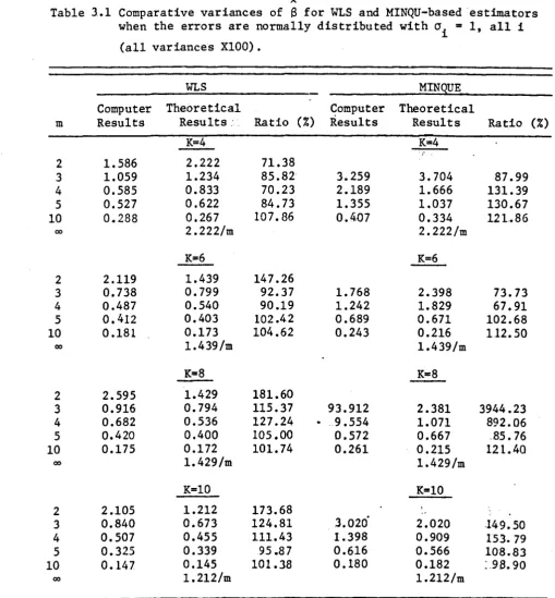
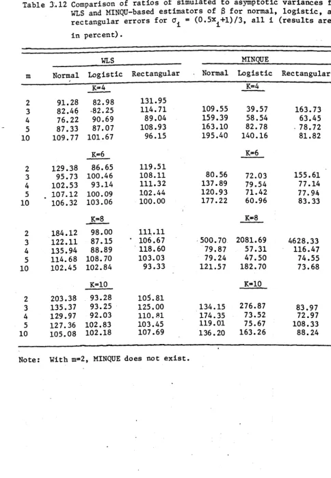
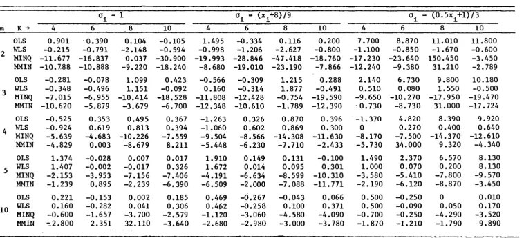
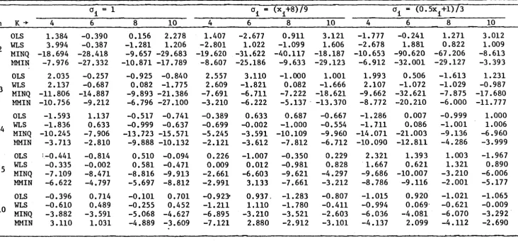
Chapter 3 provides a comparison of the theoretical results based

on Chapter 2 with simulated small samples results. These simulated and

theoretical results are based on WLS and MINQU-based estimators for normal

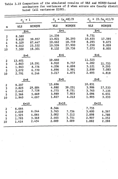
and non-normal distributions. A Monte Carlo comparison of the modified

MINQU-based, OLS and WLS estimators is also given.

In Chapter 4, we present the theoretical developments of the

Posterior Likelihood (PL) methodology and their theoretical properties.

"

Some theoretical results about the ~ and the variances are obtained

using Gamma prior likelihoods for the regression model. A comparative

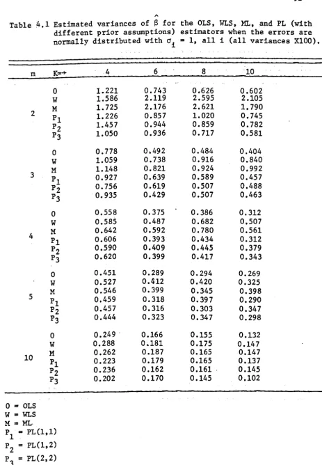
empirical study on the basis of OLS, WLS, ML, and PL is also presented.

In Chapter 5, we present adaptive procedures for estimation. A

review of existing techniques for testing equality of variance~ is

parameters after using preliminary tests of variance equality are

discussed and empirical results on the adaptive estimators are also

provided.

Chapter 6 provides a review of the literature on multiple

comparisons and adaptive estimators using multiple comparisons procedures.

Empirical comparison of these adaptive estimators with other estimators

are also presented.

In Chapter 7~ we examine the effects of "errors in variables" upon

the different estimators. Empirical comparisons are again provided.

Finally, in Chapter 8, we present an overview of the results and

CHAPTER 2

LARGE SAMPLE PROPERTIES OF WLS AND MINQU-BASED ESTIMATORS

2.1 Introduction

The main purpose of this chapter is to determine the large sample

properties of WLS and MINQU-based estimators for the linear model. The

theoretical results of this chapter will be used in the next chapter for

comparison with the simulated small samples results.

In Section 2.2, we state a general Theorem 2.2.1 for the WLS and

MINQUE cases with normally distributed error terms, with zero means and

variances Oii for the n

i observations corresponding to Xi' i-l, ••• ,k.

We also develop several lemmas prior to prove the main theorem.

In Section 2.3, we present the complete proofs of Theorem 2.2.1

for the WLS and MINQUE cases.

In Section 2.4, we present and prove Theorem 2.4.1 for WLS and

MINQU-based estimators for non-normal distributions. Two new lemmas

are also derived to prove the results of Theorem 2.4.1.

To check the applicability of the above theorems for WLS and

MINQU-based estimators for normal and non-normal cases, we consider some special

cases of the above theorems in Section 2.5. In particular, we consider

the special cases when all the variances are equal and all the n

2.2 Asymptotic Results

In the next two sections, we shall state and prove theorems which

give the expected value and variance of WLS and MINQU-based estimators

for ~ in the linear model.

Theorem 2.2.1

Consider the linear model

Y = XJi

+

.i,

k

where Y is a vector of n =

L

i observations, X is a known matrix of i:ll1

order n x p, ~ is a vector of p unknown parameters and E is a vector of

n. Further, assume that

(2.2.2)

(i) The WLS Case

The WLS estimator is

(2.2.3)

where

"

0'11I n

1 0

"

V - (2.2.4)

0

'a

" -1 n

i

- 2

A -2

Then E(~) =~; and to terms of O(n ),

where

A

o (pxp)

=

(pXk)

o

and x has rows x., (i=1, ••• ,k).

-1

(11) The MINQUE Case

o

(kxk)

The MINQU-based .. estimator for 8 is

A

where V =

o

n and the MINQUE of (J = -..".;.:....~

11 n

i (n-2)

2 -1 - 2

where 5

=

'0

kk~

l

-

(2.2.5)

x' (2.2.6)

(kxp)

(2.2.7)

A A 2

Then E(~) =~, and to terms of O(n-.),

where t •.

. 1J

2 2 -1 -3 0ii 0jj ]x'Ao + O(n .).

,. ,. ) 1 -1

- cov(a •. ,a •. and g .• - x. Ao x .•

11 JJ 1J -1 -J

(2.2.9)

In order to prove the results of the above Theorem 2.2.1, we first

establish several lemmas.

Lemma 2.2.1

If the distribution of

i

even function of

i

Proof:

1 Since P(~> 0) -

2

Let !l. == -

i .

. : E[ig(f)]

=

Lemma 2.2.2

(2.2.10)

V-I = V-I _ V-1(V_V)V-1 + V-l(V-V)V-1(V-V)V-1 0(V~~)3}.

A

Proof of Lemma 2.2.2

Directly:-~-1_V-1 __ V- 1 (V_V)V- 1

Also

so

-1 A -1 -1 A -1 A A _ I

and using

*

=

-v

v (v-v) v

The result follows directly by using

**

*

Lemma 2.2.3

When V is estimatee by WLS,

E(VUV) - VUV + 2

a .. u ..

, [ 2 ] d1ag • 11 11

n.

1

where U is a known n n matrix with sub-matrices u .• of order n. x n.; and

1J 1 J

A

V is given in (2.2.4).

Proof:

vuv

as 1,J e ement 1S - cr •• cr .• u •. an V - d1ag cr .• ;

11 JJ 1J 11

,.

E(cr .. ) - cr •• ,

@

a .. a.],

t ₁₁ JJ

E

~

..

i]

-11 jj

Ear(~

o~,

11 1

and the result follows since

... 2

var(o .. ) a 20 .. /n .• 11 11 1

Lennna 2.2.4

When V is estimated by MINQUE,

no ..

where Bl - liiij Cij], B2 - diag

~iiwiiJ,

<n~~)

J

1

k

and a ..

r

U is a known matrix of n x n with sub-matrices u

ij of order ni x nj and

, /

o

"

V

=

o

"-The MINQUE of a

ii is given"in (2.2.8).

Proof:

E(VUV" ") has the diagonal e ements E uiia1 ( , , 2

ii) and off-diagonal elements

E(Gii) == _{a ii since HINQUE's are unbiased.}

10utine calculations show that

-{I 2}

+ 2na _{i t} a . - - - -_n

i n-1

(2.2.15)

and

C C ( " " ) = 2(n-2)-2 t ij = ij == _{ov aii,ajj}

(2.2.16)

it follows that

Lemma 2.2.5

Consider terms of the form

u -

Tll T12

....

·

where T = _{T2l T22}

·

(nxn)

·

Tkl

...

k is a matrix of known terms, Tij is (n

i x nj) and n -

L

O'llI

nl 0

" " "

H

=

=

.

,

0 _O'kkI

~

(2.2.17)

and

=

=

Also V is the WLS estimator of V.

Then E(U) = 2VDT~V

where _Tll~l

T~ is a block diagonal matrix, T~ =

( 1 f\

M

=

-.1"

Proof:

and D =

o

o

"1 - I

~ ~

o

th

U has (r,q) block u

n

r _ 2

Now (n -1)0 =

r

n r

=

r

=

r

i r ri i=l

~

,

n

r

r

(E

rs-s-q i=l r i r r

thus E (U )... E

--L.:=-=~-=-:(-n-_-=l~)--J..----rsq r

L..

If r of s of q

- cr T cr I • rr rs sq sq

or r - s, r of q ====> E(U _rsq )

=

if a of b,

if a

=

ErE E'

lE

21l

L-r-r _{r i r r}

= - - -

r

ErE E'

L-r-r

lE

-n

21~

=

[en

(n +2)(n -1) 2

r r

= - - - c r _n

r rr

(2.2.18)

th . ]

Substituting these values (2.2.18) will be as

2(,2

E ( ) _urrr

₌

~I

r r

E (u ) ... 0, when r ..; q. rq

E(U ) .. rq

..

2(i

n -1

r

20'2 T rr rr M

n -1 rr·

r

_ L

n -r

:. E(U) .. 2VDT6.V.

Lemma 2.2.6

Consider terms of the.form

U .. HT(i!'-V)

where T

=

Tkk

when r ... q

k is a matrix of known terms, Tij is (n

i x nj ) and ri."

l

o

(2.2.19)

H

= V-V,

V

=

A "

and V has O'ii in place of O'ii.

"-The MINQUE 0 f a ii (M) is given in (2. 2. 8) and

E

=

nx1

[~

)

Then E(U)

=

where

ii

=

where C

=

[{nr(~-2)

(n -1) }

- (n-1) (n-2)

T~ is the block diag matrix, T~

-o

M ,. (I -

1-

rr n - -_r and D

=

o

Proof:

o

·1

- I

,

~ ~

U has (r,q)th block u ,.

I

(a

rq s rr rr rs -s-q sq sq

n

v r rr

where

0

r

----E!.T M

2ci

[

n -1

l

(n-I) (n-2) _

r r

E(U)

=

Lennna 2.2.7

If X is a n x p matrix [

~

=

g1I _n 0 1

-1 Then diag(XA X')

-0

0

.

~

and A

=

o

(2.2.20)

1 . , . th

where gi ... ~'A~ xi' where the ni_1+1,ni_1-2, ••• ,ni rows of X are xi'·

Proof:

x ' -1

x '

-1

Since X ..

x ' -2

(nxp)

1.1 (n

1x1)

1:.

_z

X

=

0

where

x ' -1

x' ==

(kXp)

.

~'.

Hence

=

x ' -1

.

0

_ L x'

(nxk) (kXp)

4:

(~X1)

,

.~~' (Z.2.21)

1

and 1

-, -1 xl A xII

- 0 - n

o

1

1

x 'A-1x I -2 0 -2 n

2

o

o

o

, by definition.

Lemma 2.2.8

If M is the diagonal matrix

1.1

0

M1 0 n1x1

1.2

M= and L =0 n

2x1

0

_~

o

where M

=

1-

=

Proof:

In matrix ML, all the terms on the block diagonal are alike, so it

will be sufficient to show that

ML=

Hence ML

=

Lemma 2.2.9

where

o

hll (kxk)

M 1 _rr-r

=

where M 1

=

rr-r n

r 1

- -- 1 1')1 - 1 - 1 = O.

n -r-r -r - r -r

r

Proof:

From (2.2.21), X

=

-L_ -1 -1. -1 hence X'V IffV X

=

(2.2.24)

But

so that (2.2.24) reduces, as required, to

(2.2.25)

2.3 Proof of Theorem 2.2.1

(i) The WLS Case

The linear model is Y ~

XB

i.

o

A

where V

=

....

Since V is an even function of il,.·.,in , it follows that

(X'V-lX)-lX'V-l is an even function of i l ' ••• '~. Thus, applying

Lemma 2.2.1,

Now

(2.3.1)

Let EE'

_-

=

_-

=

(2.3.4)

"'-1

Applying Lemma 2.2.2 and substituting the values of V into the

.... -1 term (X'V X),

(X'V-LX)

=

=

and

then

Let

V -

=

x'V-lx

=

X'V-l(V-V)V-lX ~ x,v-~v-lx - AI'

X'V-l(V-V)V-l(V-V)V-lX - x,v-~v-lHV-lx - A

. . 2'

~

~l

~lArA~l

A~lA2A~1

~lAl~lAlA~l

+

(2.3.5)

Substituting the values of (2.3.6) up to 0(H 3) in (2.3.4)

where

Thus

(2.3.8)

which we write as

....

Var(~) - Term I + Term II. _(2.3.9)

We will now examine these two terms separately.

Term II

=

=

E[FX'V-1{I-2HV-1+3(~V-1)2+O(H3)}XF]

_ E[F{X'V-1X-2X'V-~v-lX+3X'V-l(HV-l)2X}F]

=

E[F(~1_2A1+3A2)FJ

-1 -1 -1 -1 -1 -1 -1 2 1

=

+ ~ AlAO -AO A2AO +Ae (AlAO ) +0 (H )}]

(2.3.10)

Then, Term I = E[FX'V-1(l-HV-l)Q(l-HV-l)'V-l XF]

=

E[~lX'V-lQV-lXA~1_~lX'V-~V-lQV-l~1_A~lX'V-lQV-~V-1XA~1

+ A-lJLA-lX'V-lQV-lXA-l+A-lX'V-lQV-lXA-lA A-l+o( -3)]

o

Then we must evaluate the following terms:

E(QT1~)' E(~T1Q) in Term I.

E(A

2) - E(X'V-~V-~V-1X)

_ X'V-1E(HV-~)V-1X.

But

E(HV-~)

=

-1

Applying Lemma 2.2.: with U =

v[ai~In

1

..

E(HV-~)

i1 - V

By (2.2.21) this becomes

(2.3.11)

(2.3.12)

By Lemma 2.2.9, this reduces to

(2.3.14)

Applying Lemma 2.2.3 with

rr

we obtain

(2.3.15)

where gi

=

~'A~l~

Substituting (2.3.13) and (2.3.15) into (2.3.10) we get

Now we shall evaluate some terms for Term I (2.3.11)

E(~lX'V-1QV-1~1) _ ~lX'E(V-1QV-1)XAQ1

=

-1) - 0

= ~lX'V-1(V_V)V-1XA;1 _ 0

using Lemma 2.2.5

-1 -1 -L -1 -1 Similarly E(A_O X'V QV IffV XAO)

=

(2.3.16)

(2.3.17)

(2.3.18)

Let _{T -}_ -lXA-lX'V-l _{V 0}

Applying Lemma 2.2.5

(2.3.20)

Similarly

(2.3.21)

Substituting the values of (2.3.17)-(2.3.20) in Equation (2.3.11) we

obtain

_•

-1, "-L -- -1 -1, -1 -3 Term I

=

where

and

Lr

1 n1

D

=

O '1 - I

n_{k ~}

-1 -1 -1 TlI

=

XAa

M-Using Lemma 2.2.7, Equation (2.3.23) beco~es

M1

0

(2.3.22)

o

.~

glM _n 0 1

T = V-I

-1

V (2.3.24)

!J.

0 gkM _n k

glM _n

1 ₀

2 n10"11

(2.3.25) • DT

-••

!J,-gkM

~

0 2

~O"kk

Using Lemma 2.2.8

-x x' - 0 (2.3.26)

o

Using the results of (2.3.25), (2.3.26), and (2.3.17) in (2.3.22)

, -3 Term I ? 0 + O(n ).

(2.3.27)

Substituting the results of (2.3.16) and (2.3.27) in (2.3.9), we get

(ii) The MINQUE Case

Taking the linear model (2.2.1)

y

=

xS

i

o

" where _V

₌

"

Using the UnTQUE of O"U·given in (2.2.8), it follows that, as before,

E(~)

=

~.

Now we wish to evaluate

The results up to (2.3.11) are the same, so we ~ill evaluate Terms

I and II. Starting with Term II

E(A) ..

E[X'V-~V-~-lXJ- X,v-lE[HV-~JV-~

2 .

.. -1

Applying Lemma 2.2.4 with U - V , we get

E(HV-~) ~ diag[(Ci~+2Wii)

I

- 2T~ say

where tii is given in (2.2.15).

(2.2.28)

-1 -1 -1 -1 -1 -1 Likewise E(~AO AI)

=

Applying Lemma 2.2.4, it follows that

(2.2.29)

-1

where gij ..

:s}AO

Substituting (2.3.28) and (2.3.29) into Term II (2.3.10)

(2.3.30)

The results for Term I are as follows:

(2.3.31)

Using Lemma 2.2.6, the remaining terms of Term I «2.3.18)-2.3.21»

will be as follows:

1 -L_ -1 -1 -1 -1 -~A-1

E(A~ X'V ~V QV

XAo)

=

E(~lX'V-1QV-1HV-1~1)

2A~lX'CDV-~1

E(~lA1~lX'V-1QV-1XA~1)

2A~lX'CDT~XA~1

and

E(A~~'V-1QV-~~lA1A~1)

=

2A~~'CDT~XA~1

-1 -1 -1 where T~

=

(2.3.32)

(2.3.33)

(2.3.34)

(2.3.35)

(2.3.36)

Substituting the values of (2.3.31)-(2.3.35) in (2.3.11),

(2.3.37)

o

o

where D

=

o

DT

_t:.

=

o

o

n CDTt:.

=

o

o

1 (2.3.38)

- (n-1)(n-2)

o

Using Lemma 2.2.8 (ML

=

x'cDv-IMx -

xL'CDV-~'

-

o.

Thus, using the results of (2.3.38) and (2.3.39) in (2.3.37)

. -3

Term I

=

A

So var(~}

=

A _ -1 -1· ( / 3 ., -1 -1 2 2 -1

2.4 Non-Normal Case

Theorem 2.4.1

Consider the linear model

y=xS+i

k

where Y is a vector of n

=

L

order·n x p, ~ is a vector of p unknown parameters and

i

n. Also Eij ~ _{ID(Q,crii,yi ) where Yi is the measure of kurtosis. It is}

assumed that the distribution of the Eij is symmetric.

(i) The WLS Case

As before, the estimator is ~

=

crllI

nl 0

"

n i

- 2

" _and

L

where

v-

ii .. (Yij-Yi ) /(ni-l).

" j=l

0 crkkI_nk

"-Then E (~) =~, and

(2.4.1)

(ii) MINQUE Case

As before, the estimator is ~

=

o

and the ~INQUE of

cr

ii is given in (2.2.8). Then E(~)

=

(2.4.2)

where, again by routine calculation,

(2.4.3)

and

(2.4.4) ..

In order to prove Theorem 2.4.1, we first prove the following two

lemmas:

Lemma 2.4.1

,.,

When V is estimated by WLS

(J u (2+y)

( 2 1

E(VuV)

~

o

....

v

=

l

o

Proof:

.... .... th ~~ .... .... VUV has (ij) element

=

.... ....

where V

=

Now,

and

(ni-l~ (n i-3) 3

n i

2

(ni -3)O'ii 2 +0' (n -l)n ii '

i i

A "

Further, E(criicr_{j j})

=

zero. Thus E(VuV) has the (ij)th element

=

I I

2

=

" " • E(VUV)

Lemma 2.4.2

"

When V is estimated by MINQU,

U is a known matrix and

o

" V=

o

A

cr

ii being the MINQU estimator is given in (2.2.8).

Proof:

The proof is on the same lines as for Lemma 2.4.1.

.

,

if i;'j

where i=j.

A A A2

E(VUV) has diagonal elements E(UiiOii) and off-diagonal elements

It follows that

. and

Using the values of (2.4.3) and (2.4.4), we obtain

(2.4.7)

(i) Proof of Theorem 2.4.1 (WLS Case)

Given the symmetry of the

ii

arguments that

A A

E(~) - ~.

For the variance, the results up to Equation (2.3.11) are the same. We

now evaluate Terms I and II. Starting with Term II,

-1

(2+Yi ]

... x diag

r

-1

Again using Lemma 2.4.1, with U ... V and Lemma 2.2.9, we obtain the

-1

expression for E(~Aa ~) as follows

(2.4.9)

In this case, all the terms of Term I vanish. Substituting the

values of Terms I and 11 in (2.3.9); we obtain

, -1 -3 x AO + O(n ).

(ii) Proof of Theorem 2.4.1 (MINQU Case)

Given the symmetry of the

ii

"

For the variance, the results up to (2.3.11) are the same and the

terms of'Term I vanish by arguments similar to those in

(2.3.31)-(2.3.39). So

var(~)

=

Now we evaluate Term 11.

. -1

Using Lemma 2.4.2 with U·· V

E(HV-~)

I

where the value of tii is given in (2.4.3).

Likewise, applying Lemma 2.2.9 and Lemma 2.4.2,

where t

ij is given in (2.4.4).

(2.4.10)

(2.4.11)

(2.4.12)

Substituting the values of (2.4.11) and (2.4.12) into (2.4.10) _,

_,

Var(~) A =

Aa

+2Aa

-2Aa

. O'iiO'jj

2.5 Special Cases of the Theorems

•

In order to examine the effect of the second order terms, we consider

the following special case.

p

=

=

and

It follows that

o

-1 -1

Aa

=

x'v

=

Hence gi

=

x'Aa

In.

Now we evaluate the variances for each case.

Example 2.5.1

Using WLS and assuming normality

V(~) A ... Aa +2Aa x diag -2--1 -1 {1 ( _{aii-nigi x} )} ,-1

Aa

2

a

=

2" -

n n a ka

_

o~

+

2:{

{k~l}

+

0(0-3)

_

~2

{l

+

2(~-1)}

+

O(n -3).

for i=1,2, ••• ,k.

x' _

~ I~

I

l. ni vii - n a •

i-1

Example 2.5.2

Using MINQUE and assuming normality

wh~re tii and t_ij are given in (2.2.15) and (2.2.16).

This becomes

Var(~

=

(i

+

i/

"'M n n 2 Lk n-2 (n-l) (n-2) (1 -'

[

k.k _ k2

J

+

= (12

+

+

+

n n(n-2) - n(n-l) (n-2) - n(n-2) n(n-l) (n-2)

_ (12 [1

+

l

+

n (n-2) (2.5.2)

Example 2.5.3

Using WLS without assuming normality and taking all Y

i

=

(12 2 3

- -n

n

Example 2.5.4

Using MINQUE without assuming normality and taking. all Y

i

=

where tii and t

ij are given in (2.4.3) and (2.4.4) respectively. It··

follows that

(2.5.4)

It .is apparent that the MINQU-based estimators have higher variances,