Suspended sediments under plunging waves

(1)

SUSPENDED SEDIMENTS

UNDER PLUNGING WAVES

Bachelor thesis

Mick Poppe

(2)

Suspended sediments under plunging waves

Thesis for the bachelor Civil Engineering at the University of Twente

Concept report

Author: Mick Poppe (s1237470) [email protected]

Supervisors: Dr. ir. J.S. Ribberink Msc. J. van der Zanden

Place: Enschede, The Netherlands

Date: 20 August 2014

Photo front: Science of the Surf, made by Tim Scott

(3)

(4)

Abstract

Knowledge of the coastal morphology is critical for coastal safety. Unfortunately, knowledge is limited when it comes to sediment transport under irregular breaking waves. In this thesis it is aimed to improve the understanding of suspended sediment concentrations under regular plunging breaking waves. The variation of the sediment concentrations over time and the cross-shore direction is studied, as well as the relation with the water velocities and the net sediment transport. Empirical models are used to describe the concentration profiles of the sediments.

Experiments were executed for two months in the CIEM wave flume in Barcelona (Spain). Over a bed development time of 90 minutes a transverse suction system is used to determine the sediment concentrations in the water. Other measuring equipment was used to measure water velocities, bed development and more. Data from especially the transverse suction system is used for analysis.

The sediment concentrations decrease from high concentrations in the water at the top of the breaker bar to a less high concentration in the water at approximately 3 meters from the top. Beyond 3 meters from the top of the breaker bar the concentration decreases rapidly and hardly any sediments are found higher in the water column. Over the height the concentrations in general decrease, of course. However, just before and after the breaker bar higher concentrations can be spotted high in the water column, most likely caused by the water velocities and wave actions at these points. The suspended concentrations are also compared to the net sediment transport and show places were sheet flow can occur With empirical models it is possible to fit a function on the suspended sediment data. The parameters of these models show expected trends when looking over the cross-shore position. However, over time there is hardly any trend visible. A timespan of 90 minutes seems not enough to see substantial changes in the development of the models parameters.

(5)

Preface

Two months I spend in Barcelona doing experiments for this bachelor thesis. After this it took approximately another month to finish this report. It was never my plan, and still isn’t, to work at a university or some other research institute. Instead of that, I rather see myself working at a ‘normal’ company. However, during these two months I found that doing scientifical research is a lot more than only sitting behind a desk and draw conclusions based on some data and a lot of imagination. It is doing experiments, look at the data, try to find correlations, explain trends and do some more experiments. In the end you still need some imagination to see the trends and find explanations, but I guess it’s a scientifical way of imagining. That is also what I tried to do in this thesis. I used my observations and imagination to draw conclusions.

I would like to thank the people that assisted me with this thesis; Jan (Ribberink), Joep (van der Zanden) and also Dominic (van der A). I lived two months with Joep and Dominic, and with their bad (very bad) music taste, the pasta pesto and their criticism on Mr. Scofield (who risked his own life to safe his brother from prison). I can’t imagine living another two months with them. However, as researchers I wouldn’t mind meeting them again someday. I wish Joep good luck with his PhD and Dominic with his upcoming marriage.

Mick Poppe

(6)

1 Introduction

Coastal engineers use models to evaluate the safety of the coast. These models play therefore a significant role in the safety of our coastal region and their accuracy is of great importance. When it comes to sand transport in the coastal region, the models often use the understanding of fundamental processes in combination with measurements of sediment displacements. However, these processes and measurements are usually based only on laboratory experiments where identical (or regular), non-breaking waves are repeated continuously (University of Aberdeen, 2014). Since sand transport in coastal regions is in reality subjected to constantly changing breaking waves, the models representation of the real world, and thus their accuracy, is limited.

The Sinbad project, which involves researchers from the universities of Aberdeen, Liverpool and Twente, is trying to solve this shortcoming in accuracy and improve the models. It is researching the interaction between sand transport and non-identical (or irregular) breaking waves by doing large-scale wave experiments. In May and June 2014, experiments were done at the wave flume of the Catalonia University of Technology in Barcelona (Spain). In these experiments the sediment transport is observed in conditions of regular breaking waves. The breaker type used in these experiments where the plunging breaker type. In paragraph 2.1 this breaker type is explained.

1.1 Scope

The entire Sinbad project focusses on sand transport in conditions of irregular and breaking waves. This thesis, conducted for the Sinbad project, concurs with this, but will contain only a small part of the goal. Only regular, plunging breakers are of interest in this thesis. Furthermore, instead of researching all components of the sand transport, here only the suspended sediment concentration over the water height will be analysed.

Even within regular waves randomness occurs. This randomness will make it difficult to draw solid conclusions, since there are too many variables that can cause an observed trend. To make sure conclusions can be drawn, there are two ways to analyse the data. First of all averaged data will be used to smoothen out large outliers. Second, empirical models are used to describe the sediment profiles. These models have less variables and are therefore better suitable for analysis. The empirical models will be further explained in paragraph 2.4.

1.2 Research goal & questions

In this thesis it is aimed to get a better understanding of the sediment concentration due to regular, plunging breakers. The research goal is stated as:

Improve the understanding of suspended sediment concentrations under regular, plunging waves.

To reach this goal, a question needs to be answered:

How are suspended sediment concentrations affected by regular plunging breaking waves?

This research question is directly related to the research goal. Answering this question is rather complicated, since a lot of different processes will still influence the sediment concentrations under regular plunging waves. A few sub questions will lead the research in the right direction:

a) How are sediment concentrations related to water velocities and the net sediment transport? b) Which empirical model describes the sediment concentration profile most accurate?

c) How are sediment concentrations varying along the cross-shore profile and over time?

(9)

1.3 Research method in brief

To do analyses with sediment concentrations, it is firstly important to find these concentrations. Therefore experiments are done at the wave flume of the Catalonia University of Technology in Barcelona. During these experiments regular, plunging waves are created which will suspend sediments. With suction nozzles water is sucked from the flume at different heights and by determining the amount of sediment in the sucked sample, the concentration in the water can be calculated. Therefore a concentration profile for the water can be drawn.

The sucked samples will be collected at different places and different times. Because of this, it will be possible to see the variability of this concentrations over time and place. Analysing this variability will make it possible to answer the research questions.

1.4 Thesis outline

(10)

2 Theoretical framework

In order to execute the experiments in a proper way and, just as important, to perform a correct analysis, it is necessary to have some background information about wave breaking, sediment transport, the nozzle suction system and empirical models. This background information is provided in this chapter.

2.1 Plunging breakers

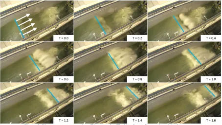
Waves can break upon the shore in different ways, depending on the wave and shore properties. One of the main breaker types is the plunging breaker, which is characterized by its arch shape (The Open University, 1989). Since wave speed depends on the water depth, the top of the wave (or wave crest) will travel faster than the water underneath when approaching the shore. At some point the wave becomes unstable and starts turning over. Then the tip of the wave, the wave jet, plunges into the trough in front of the wave. In Figure 1 a plunging in the Barcelona wave flume is shown. The time in seconds is given in the figure, together with the wave direction in the top left picture. The blue line indicates the movement of the original wave crest.

T = 0.0 T = 0.2 T = 0.4

T = 1.0

T = 1.6 T = 1.4

T = 0.8 T = 0.6

T = 1.2

Figure 1: Wave movement over time (T in seconds). The blue line indicates the original wave crest

[image:10.595.71.526.275.532.2]

In Figure 2 some important processes in the wave are schematized. With the two figures the plunging wave properties are further explained.

(11)

When the wave plunges, a part of the wave jet is penetrating the water surface and another part is reflected of the water. In Figure 1 this is visible from T=0.4 seconds. Water from the wave trough will also be splashed up due to the impact of the plunge. This is hardly visible in Figure 1, but is schematized in Figure 2. The effect is similar when tossing a rock in the water; due to the impact of the rock the surrounding water will splash up.

The splash up of both the reflected jet and the trough water will partly be overtaken by the wave crest, what happens at T=0.8 seconds. When this splash up hits the water surface again after the wave crest, it will create a disturbance area which can be seen clearly at T=1.2 to T=1.6 seconds. Furthermore, air is taken in with the penetrating wave jet, what will also boil up when the wave crest passed. This air boil up is also part of the disturbance.

A part of the splash up also stays in front of the wave crest, creating a so called surface roller. This surface roller will become smaller and partly integrate back into the wave from T=1.0 to T=1.6 seconds, until it disturbs the wave crest again and causes it to plunge again. From then, small plunges will continue until the beach. In this small scale plunging no clear processes can be further distinguished.

2.2 Sediment action

The movement of water particles, which can be caused by waves or, on a larger scale, by currents, can produce a shear stress on the sediment bed. Because of this, sediment can be displaced and the bed profile can change significantly. Figure 3 illustrates some of the main processes in the water. With the help of this figure it is attempted to describe the effect of the wave on the sediments.

Figure 3: Wave effect on sediment

So sediments are put into suspension due to shear stresses on the bed. These shear stresses can be created in multiple ways. Two of these ways are:

 Circular movement wave jet: when a wave plunges, a lot of energy is dissipated over a small distance. The wave jet will continue in the water and it will make a circular movement to the back. This circular movement will result in shear stresses at the bed and will put sediments into suspension.

(12)

larger ripples. At some point, with an increasing oscillatory velocity, sediment will not be rolling and sliding over the bed anymore (The Open University, 1989). Instead of this, sediments will suspend and will travel with the flow just above the bed, again on- and offshore. This so called sheet flow, which can be seen on the left of Figure 3, creates a small layer just above the bed with very high sediments concentrations. The sand in this Sinbad experiment require a velocity of approximately 100 cm/s to have sheet flow.

When sediments are put into suspension, they are subjected to all the flows in the water. The timing and location of the sediments is crucial for the sand transport, since water flows change continuously over time, place and strength. Such a change is, for example, noticeable when a wave runs upon the shore. The wave speed will decrease and therefore the wave height have to increase according to the law of conservation of energy. For the wave to increase in height, it needs to take in water from below. This also causes sediments to go into the wave. When the wave plunges, it will cause new flows and distributes sediments further in the water. For the timing and location the wave skewness is also important. This is the phenomena that the onshore movement of the wave crest is much more powerful than the offshore movement of the wave trough. However, the onshore movement is also shorter than the offshore one.

In this paragraph, the focus was on the so called wave induced flows. However, when looking on a larger scale, also current induced flows can be distinguished. These are simply put the average wave flows over a longer time. It turns out that waves create an onshore flow relatively high in the water column and an offshore flow, the undertow, low in the water column. This can also be seen in Figure 3. In this thesis, those current flows are of most interest, since the concentrations that are collected are also a result of multiple wave periods.

2.3 Transverse suction system

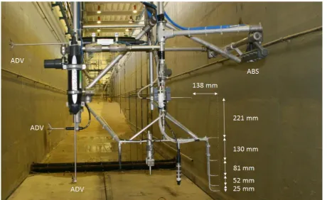
[image:12.595.72.525.495.750.2]

To measure the sediment concentration in the water above the bed, a transverse suction system is used. This measuring equipment makes it possible to collect average sediment concentrations at a certain point in the water (Bosman, Van der Velden, & Hulsbergen, 1987). Water and sediments are sucked from the flow with the help of nozzles and pumps. With the concentration in the collected sample the true concentration in the flume can be calculated. In Figure 4 the measurement frame used during the experiments can be found. The six suction nozzles are marked with white circles.

(13)

The measurement frame with the nozzles would, during waves, be under water. Each of the six nozzles is connected with a tube to a peristaltic pump at the top of the frame. Water and sediments are pumped up from a nozzle and are released into a bucket. From the sample in the bucket the weight of water and the weight of sediment is measured, so the concentration in g/L can be determined. Also the time is notated to determine whether the nozzle intake velocity is high enough. With the help of a calibration factor the flume (or true) concentration can be calculated from the sample concentration. More detailed information about the measurement with the transverse suction system can be found in Appendix C: Measuring procedure and measuring form.

2.3.1 Calibration factor β

To calculate the true sediment concentration, the sample concentration need to be multiplied with the calibration factor β. The equation for β is:

𝛽 = 1 +1

3arctan ( 𝐷₅₀

𝐷_𝑟) (2.1)

In this equation D50 describes the sediment size and Dr is a constant of 0.090 mm (Bosman, Van der

Velden, & Hulsbergen, 1987). Since the sediment size during the experiments was constant (see paragraph 3.1.1), β is constant.

2.3.2 Requirements of transverse suction system and its error sources

In order to use the transverse suction system, Bosman et al. (1987) state two important requirements:  Nozzle orientation: to make sure the nozzle collects the sediments from the flow, it should be

projected normal to the main (or ambient) flow direction. Since flows in the flume travel mainly over the length of the flume, the nozzles should be projected perpendicular to this. As can be seen in Figure 4, the nozzles in this experiment satisfy this requirements.

 Intake velocity: because of the fact that the nozzle is projected normal to the ambient flow, water and sediments will naturally not stream into the nozzle. To overcome this, the intake velocity should be at least three times the peak ambient flow velocity. Bosman et al. (1987) state that in small flumes a suction velocity of 1.5 m/s is sufficient to meet this requirement. Larger wave flumes have much higher peak velocities, but since these velocities only appear for a relatively short time, a suction velocity of 1.5 m/s is also sufficient in larger flumes. It will lead to a small systematic error, but this is negligible compared to the total error.

These two requirements should be met in order to use the transverse suction system. However, even then, still substantial errors can occur. Some general error sources are:

 Suction errors: when water and sediments are sucked from the flow, the nozzles or the tubes can be partly or fully blocked with sediments or pollutants from inside the flume. This can make a sample useless. More often the blockage is only for a short time and the sample collection can continue after a few seconds. However, the collection is disturbed so there is still an error present.

 Processing errors: to measure the amount of sediments inside the collected sample, water have to be drained, sediments are poured from one cup into another, water is added again and the samples are dried. In all of these steps sediments can be lost, creating an error.

 Random errors: since wave actions are somewhat random, there are pollutants in the flume and there are other random sources, conditions in the flume are not always exactly similar. This create a random error which can’t be avoided.

(14)

2.4 Empirical models

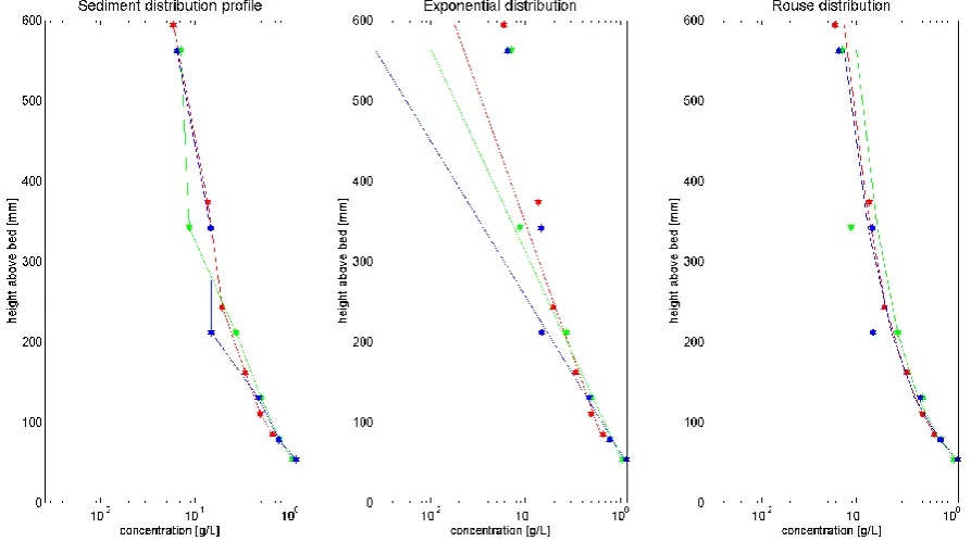
[image:14.595.76.523.151.400.2]

Sediment concentrations in grams per litre are collected at different heights in a water column. By combining these different concentrations, a graph can be made where the height is plotted against the concentration. This is a so called sediment concentration profile. Often the concentration is plotted on a logarithmic scale. Three examples of concentration profiles can be found on the left side of Figure 5.

Figure 5: Sediment concentration profile (left) with exponential model (middle) and Rouse model (right)

In the figure the concentrations of three runs are displayed. In general, the concentrations at each height are very much alike. There is only a small concentration decrease at 350 mm height for the green line and a small decrease at 200 mm height for the blue line. To do an analysis with these runs, they can be compared to each other and to other runs on different locations. With a few runs this is not a problem, but when more runs are compared, it will become harder to analyze.

To make analysis possible, even with a lot of concentration profiles, empirical models can be used. Empirical models are formulas that describe the concentration profile. The variables of such a formula can be compared to each other and so it is possible to compare different runs on a quantitative way. For concentration profiles, two empirical models are generally used. These are the exponential model and the Rouse model (Aagaard & Jensen, 2013). The exponential model can be seen in the middle of Figure 5, while the Rouse model is found on the right.

(15)

2.4.1 Exponential model

The exponential model describes the concentrations profile with a straight line on the logarithmic scale. This straight line suggests that there is homogeneous turbulence in the water and sediments are therefore more evenly distributed over the height. This occurs around the breaker zone and here it is expected that the exponential model gives a better fit. The equation for the exponential model is:

𝐶(𝑧) = 𝐶₀exp (−𝑧

𝑙_𝑠) (2.2)

In this equation z is the height with respect to the bed, C0 is the reference concentration near the bed and

ls is the so called decay length. A higher ls will lead to a steeper slope, so the amount of sediments higher

in the water column will increase. A higher C0 will result in a shift of the function to the right, which

means that there is a higher concentration at the bottom.

The exponential model will be fitted on the different concentrations by varying both the reference concentration as the decay length. A best fit is found when the total horizontal deviation is at its lowest. In previous Sinbad experiments exponential reference concentrations varied between 0.2 and 5.5. The decay length varied between 0.1 and 5.5 (Van Til, 2014). These experiments were conducted in similar conditions.

2.4.2 Rouse model

Another possibility to describe the concentrations profile is with the Rouse model. This model plots the concentration with an increasing steepness, as can be seen on the right of Figure 5. At places with lower mixing over the height, so before and after the breaker bar, this model will most likely describe the concentrations with greater accuracy. The equation that the Rouse model uses, is:

𝐶(𝑧) = 𝐶_𝑎(𝑧_𝑎/𝑧)𝑛 _(2.3)

In this formula z is again the height, Ca is the reference concentration at the bed of a height za above the

bed (normally 0.01 meter) and n is the Rouse suspension number. A lower n will increase the steepness of the fit and therefore increase the amount of sediments higher in the water column. An increasing Ca

will again lead to a shift of the model to the right, so to a higher concentration near the bottom.

With the Rouse model the reference concentration and the suspension number are both varied to find the best fit, while za is fixed at 0.01 meter. Again a best fit is found when the horizontal deviation is at

(16)

3 Research design

Now the theoretical framework is presented, it is necessary to provide some information about the experiments before going to the results. In this chapter the most important conditions and properties of the experiments and the experiment equipment is therefore presented.

3.1 Experiments

During the months May and June 2014 experiments were conducted in the CIEM wave flume in Barcelona. In 24 experiment days, 72 runs of 15 minutes were performed on 12 locations (6 runs per location) in the wave flume. The measuring equipment used for this thesis was fixed on a moveable frame, so measurements could be taken at different cross-shore positions and at different heights.

3.1.1 Experiment set-up and conditions

In Figure 6 the initial set-up of the CIEM wave flume is shown. The flume has a total length of 100 meters (however the effective length is smaller), a height of 5 meters and a width of 3 meters. Inside of the flume the following things can be found:

 Fixed beach: at the very end of the beach a 18 meters long fixed beach is found.

 Sand beach: against the fixed beach a 20 meter long bed is created with a height of 1.35 meters and a D50 of 0.24 meters.

 Sloping beach: before the 20 meters sand beach, a sloping beach is created with a slope of 1:10 and a D50 of again 0.24 meters. The total length of the sloping beach is 13.5 meters.

 Wave paddle: at the very beginning of the flume the wave paddle is found. This is used to create the waves.

All distances in the flume and this report are measured from the wave paddle in resting position. The measuring line shown in Figure 6 indicates the distances from this wave paddle.

Figure 6: Global overview wave flume with distances in meters

When the beach was created, the flume was filled with water and approximately 7 test runs of 15 minutes were conducted, while the frame was at the end of the beach. After this, the flume was drained and the formed bed profile was smoothened and then drawn on the flume wall. This bed profile formed the basis for all the experiments. More information about the creation of this bed can be found in Appendix A: Creating the starter bed.

For one series of experiments, so for six runs, two days are reserved. On the first day, 6 runs of 15 minutes are executed. At the beginning and after every second run, the bed profile is measured. The height of the moveable frame is, if necessary, adjusted before every run. It is aimed to keep the distance between the bed and the measuring equipment. After the 6 runs, the flume is drained on the same day. On the second day the bed profile is restored to the one drawn on the wall. The flume is then filled again, also on the second day, so the flume would be ready for the experiments of the following day.

The wave properties during the experiments were as followed:  Wave period: 4 seconds

 Wave height: 0.85 meters  Water depth: 2.55 meters

(17)

3.1.2 Measuring program

[image:17.595.70.531.419.701.2]

As stated before, measurements are taken over 24 experiment days. In Table 1 the measuring program of the experiments is given. Only days where runs were conducted are given in the table. The next working day the bed was restored to the start position.

Table 1: Measuring program

Date Runs Position

19 May ‘14 1 to 6 51.0 meters

21 May ‘14 7 to 12 60.0 meters

23 May ‘14 13 to 18 55.5 metres

27 May ‘14 19 to 24 57.0 meters

2 June ‘14 25 to 30 54.5 meters

4 June ‘14 31 to 36 59.0 meters

6 June ‘14 37 to 42 56.0 meters

11 June ‘14 43 to 48 58.0 meters

13 June ‘14 49 to 54 56.5 meters

17 June ‘14 55 to 60 63.0 meters

19 June ‘14 61 to 66 55.0 meters

25 June ‘14 66 to 72 53.0 meters

3.1.3 Measurement equipment

On the moveable frame many instruments were installed. Instruments of interest for this thesis are especially the transverse suction system and the ABS. Besides those, also data from the ADV’s and the profile measurements are used. The nozzles of the transverse suction system and their distances, the ABS and the ADV’s can be found in Figure 7. The profile measurement equipment is not visible.

Figure 7: Relevant measuring equipment on frame (original photo by Van Der A)

(18)

The acoustic backscatter system, or ABS, is also marked in Figure 7. The four sensors the system has all sent an acoustic signal and measure the reflection. The amount of the signal that is reflected is a measure of the amount of disturbances in the water. When the signal is reflected of the bed, the reflection is much higher and therefore the distance from the sensor to the bed can be determined. Since the distance from the ABS to each of the nozzles is known, the distance from the nozzles to the bed can also be calculated. It is this distance that is of interest in this thesis.

The acoustic doppler velocimeter, or ADV, is used to measure water velocities at a single point in the flume. Because three of them were used, the velocities at three point are known. Only the maximum, minimum and average water velocities are used in this thesis to explain the sediment concentration profiles found with the transverse suction system.

Profile measurements are used only for displaying purposes and to calculate the net sediment transport. This net sediment transport is also compared to the sediment concentration profiles to check for similarities.

3.2 Data analysis

After the experiments are conducted, the data is analyzed. First of all, the sample concentration is converted to the true flume concentration by using equation 2.1. After this, the distance above the bed can be calculated with the data from the ABS. The next step is, before starting with the analysis of the data, the cleaning of the data.

3.2.1 Data cleaning

The data cleaning can be separated in two parts, namely the cleaning on a quantitative basis and the cleaning on a qualitative basis:

 Quantitative cleaning: quantitative cleaning is done mostly by two requirements. First of all, the nozzle should be located at least 10 mm above the bed. This is necessary to be able to use the empirical models that are described in paragraph 2.4. Second, the minimum suction velocity should be 1.5 m/s, as described in paragraph 2.3.2. When these requirements aren’t met, the data is excluded from the analysis.

 Qualitative cleaning: the data that comes through the quantitative cleaning is subordinated to the qualitative cleaning. Here, all concentration profiles of one location are plotted together with the exponential and Rouse fit. Also notes of abnormalities that were taken during the corresponding runs are gathered. All abnormalities in the plots of the profiles of the fits are compared with the notes and if there is a reason to doubt the outcome of the sample, this data is also excluded from the analysis. Of course, this qualitative cleaning is rather subjective. The cleaning of the experiment data can be found in Appendix D: Cleaning the experiment data.

3.2.2 Analysis of the data

(19)

4 Research results: sediment concentrations

Now that both the theoretical background and the research method are clarified, the results of the experiments and the analysis of these result can be presented. This is separated over two chapters, this one and the next one. In this chapter sediment concentrations are discussed, while in the next chapter the empirical models are found. Notice that the data used is already cleaned. More about data cleaning can be found in paragraph 3.2.1 and Appendix D: Cleaning the experiment data. All the concentration profiles of the experiments can be found in Appendix E: Concentration profiles for all locations.

4.1 Bed forming

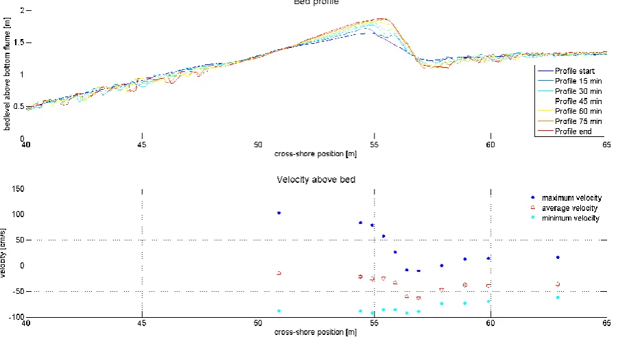
[image:19.595.74.525.305.551.2]

Soon after the first wave plunges in the wave flume, sediment clouds can be spotted in the water. It are these sediment particles that are sucked by the transverse suction system. Together with sediments that are transported as bed load, the sediments can change the bed profile substantially. In Figure 8 the development of the bed profile can be seen in combination with the horizontal water velocities measurement with the ADV’s. In this figure the positive velocities are in onshore direction, whereas the negative velocities are in offshore direction. Notice that the cross-shore position is the distance from the wave paddle, as explained in paragraph 3.1.1. The velocities are taken at an average height of 150 mm above the bed.

Figure 8: Changing bed profile with water velocities 150 mm above the bed

When looking at the bed profile, there are a few things that attract attention:

 Growing breaker bar: the breaker bar grows from 1.65 meters above the flume bottom to 1.87 meters above the flume bottom in 90 minutes. Furthermore, the top of the breaker bar shifts in the same time about 0.8 meters onshore. Water velocities are very important for sediment transport, since the transport is proportional to the water velocity to the third power (𝑞_𝑠 ≡ 𝑢3_).

Looking at the water velocities around the breaker bar, it can be seen that high positive velocities exist offshore of the breaker bar. These onshore velocities are higher than the offshore velocities, and therefore an onshore movement of sediments is expected here. Just onshore of the breaker bar negative velocities dominate near the bottom and most likely transport sediment offshore. Both the velocities onshore and offshore of the breaker bar create a growing breaker bar, since both velocities transport sediments towards the breaker bar. The velocities are a result of the wave action in this area, as explained in paragraph 2.2.

(20)

more sediments. This makes it therefore possible to smoothen out ripples or other discontinuities. When looking onshore of the breaker bar, first bigger ripples and then smaller ripples occur. This is also expected since the water velocities are decreasing closer to the shore. No velocity measurements are available offshore of the breaker bar, but the ripples there suggest that the velocities are lower than around the breaker bar.

 Breaker trough: the valley behind the breaker bar, the breaker trough, gets deeper when the time passes, creating a steeper slope at the onshore side of the breaker bar. When looking at the water velocities at this point, it can be seen that, at the bottom, the velocities are always offshore. This is the so called undertow. This undertow keeps moving sediments from this trough to the breaker bar, while no offshore flow is present to transport sediment back. It seems like this causes an increasing valley.

While the water velocity just above the bed is important for the bed forming, it is important to notice that there are many other processes that influence the sediment transport.

4.2 Suspended sediment concentrations

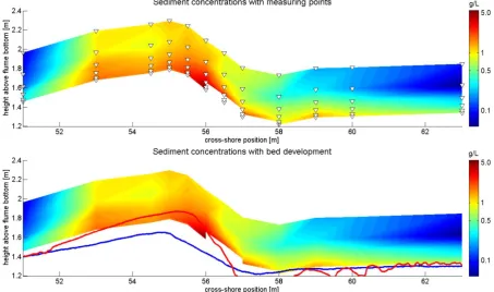
The concentration of sediments in the flume will vary over time and place. Figure 9 shows the average sediment concentration in the flume. Since on each location six runs are conducted, the average sediment concentration exist of the average value of these six runs. This method disregards the effect of time, but makes the concentration less sensitive for outliers.

In the upper plot of Figure 9, the concentration is plotted together with the locations of the nozzles in the flume. These locations are indicated with a white triangle. As can be seen, nozzles are located closer to each other nearer to the bed. The bottom plot of Figure 9 shows the concentration again, but now with the bed. The blue line indicates the initial bed, while the red line indicates the bed after six runs. The two plots are separated from each other to keep it orderly.

[image:20.595.70.524.460.728.2]

The colour spectrum of the sediment concentration is plotted on a logarithmic (log10) scale. For convenience for the reader, the colourbar on the right side displays the concentration in grams per litre.

(21)

Around the breaker bar the highest sediment concentrations are found, from 5.36 g/L near the bottom to 1.43 g/L at the highest nozzle. The lowest concentrations are measured at the beginning and the end of the measuring area, with a concentration near the bottom of 0.22 g/L and a concentration at the highest nozzle of not more than 0.06 g/L. The mean concentration near the bottom is 1.33 g/L and at the highest nozzle 0.67 g/L. Note that these numbers are sensitive for measurements errors and are only presented here to show the order of magnitude of the concentrations.

According to the measurements, concentrations of 1 g/L or more are mostly limited to an area of approximately four meters wide. Away from the breaker bar this concentration is only reached at the bed. Three meters away from the top of the breaker bar in either direction there are hardly any sediments in the water. The effect of the breaking wave therefore seems to be rather local.

Instead of focusing on the amount of sediments, it is also possible to focus on the spreading of the sediments only. In Figure 10 it is aimed to underline this spreading by dividing all the concentrations by the concentrations near the bed.

Figure 10: Deviation of sediments to the lowest nozzle

When looking over the height of a water column, the general trend is, of course, a decreasing concentration over the height. However, it can also be noticed that in parts of the experiment area the concentration seems to increase over the height after it has partially decreased. This is rather unusual, because for sediments to be higher in the water column it need to have more energy. Since lower particles doesn’t seem to have that energy, this phenomenon can only be explained when the particles are not transported only from the bottom up, but also from the side or from the top down. This is further discussed in the next paragraph.

(22)

4.2.1 Concentrations related to water velocities

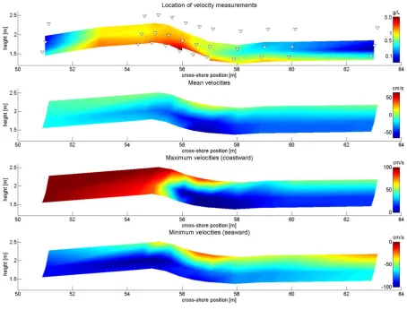
[image:22.595.70.525.171.517.2]

When the sediment concentrations are related to the water velocities, it might be possible to find some indications why the concentrations are high at certain points and lower and others. In Figure 11 the sediment concentrations are therefore plotted together with the mean, maximum and minimum velocities. In the upper plot white triangles indicate the location of the ADV’s. Note that they are located over a greater height then the concentration measurements. The highest concentration measurements don’t correspond to the highest velocity measurements.

Figure 11: Velocity measurements

According to Figure 9 and more importantly Figure 10, there are two places that are interesting for their distribution over the height:

(23)

 53 meters – 55 meters: in the area between 53 meters and 55 meters it can also be seen that concentrations tend to increase high in the water column. Around 55 meters, so around the top of the breaker bar, this effect is best visible, and it decreases the further it gets away from the breaker bar. It would be expected that, similar to the first place of interest, there is an offshore flow high in the water column that spreads the sediments from the breaker bar offshore. However, looking at the mean velocity measurements, no such trend can be observed. Actually, if there is a trend at all, the opposite is true. Maybe the high concentrations from 53 to 55 meters are not so much current induced (from the mean velocities), but more wave induced (indicated by the maximum and minimum velocities). Perhaps that sediments are put into suspension in the wave trough (minimum velocities), and move onshore again in the wave crest (maximum velocities). Since the onshore velocities are greater higher in the water column, maybe more sediments are transported high in the water, what would explain the increase in concentration. This however wouldn’t explain the fact that the concentration seems to decrease away from the breaker bar.

When comparing the water velocities to the sediment concentrations of Figure 9, there are some interesting relations:

 High concentrations breaker bar: the high concentration around the breaker bar may be explained with the help of the maximum and minimum velocities. High onshore velocities occur at the sea side of the breaker bar, moving sediments towards the top. The high offshore velocities at the coast side of the breaker bar, most likely caused by the plunging wave here, also moves sediments towards the top of the breaker bar. Both flows are probably responsible for high concentration at the breaker bar. Because there are also high offshore velocities at the sea side of the breaker bar, also high concentrations can be found at the sea side of the breaker bar higher in the water column.

 Low measured concentration offshore: at 51 meters, there are high offshore velocities, but the amount of sediment in the water is limited. It is possible that high velocities start just before this point and therefore sediments are not distributed over the water column very good yet, but this can’t be controlled since no velocity measurements are taken from before 51 meters. Another, more likable, explanation is that the velocities here are so high that sheet flow occurs. With the sand used during the experiments, sheet flow occurs at a velocity of approximately 100 cm/s (Van der Zanden, 2014). In Figure 8 and Figure 11 it can be seen that at 51 meters the velocity overtakes 100 cm/s, so sheet flow is possible.

4.2.2 Concentrations related to net sediment transport

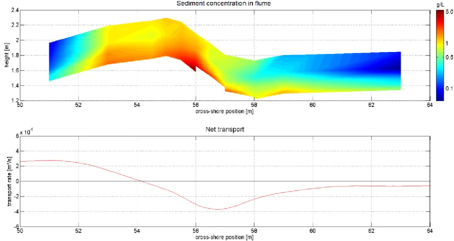
The distribution of the sediments is, to a certain level, explained with the help of the velocity measurements. The next step is to compare the sediment concentrations to the net sediment transport to find relations between these two. This is interesting, because eventually it is the net transport that is more important for the coastal safety. In Figure 12 the net sediment transport is presented. The transport is calculated by using the initial and final area under a bed profile measurements and check how much sand is missing.

(24)

[image:24.595.69.524.134.375.2]

In the figure it can be seen that net transport rates vary along the cross-shore position. Before approximately 54 meters in the cross-shore position the net transport is directed onshore, while after this point it is directed offshore. In Figure 13 only the mean transport is shown in combination with the sediment concentrations. With this figure the concentrations are compared with the net transport.

Figure 13: Sediment concentrations with mean net transport

There are three points of interest when looking at the net sediment transport:

 Maximum transport: around 51 meters in the cross-shore position the maximum transport is found. Notable is the fact that there is hardly any sediment measured in the water here. Initially, this is against expectations since there should be a lot of sand in the water to have a high transport. However, as suggested in the previous paragraph, it is also possible there is sheet flow at this location because of the high velocities. The high sediment transport contributes to the suggestion of sheet flow around this point. Since the onshore velocity is higher than the offshore velocity, more sand would be transported onshore.

 Zero transport: at approximately 54 meters there is no transport, but there are a lot of sediments in the water. From both sides sediments are transported to this point, what could be the reason of the high amount of sediments here. The sediments could pile up, making the bed grow rather fast. However, in the water itself the sediments can perhaps also pile up, causing rather high concentrations here.

(25)

5 Research results: empirical models

Empirical models to describe the sediment concentrations have only a few variables and are therefore more suited for further analysis. In this chapter the exponential and Rouse model are applied on the concentration data of the experiments.

5.1 Fitting the models

The two empirical models can be fitted on a sediment concentration curve, as explained in paragraph 2.4. The fitting process for the exponential and the Rouse model is quite similar, by simply varying two parameters and see when the total deviation is minimum. For the exponential model the reference concentration and the decay length are varied, while for the Rouse model the reference concentration and the suspension number are varied. Both models are fitted like that on all the data.

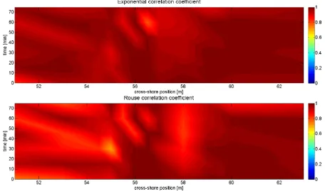
[image:25.595.72.525.325.585.2]

5.1.1 Fitting to all data

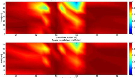
Figure 14 shows the correlation coefficient of both models. On the x-axis the cross-shore position in the wave-flume is plotted, while on the y-axis the time can be found. Since there are 6 measurement of 15 minutes on each location, a total of 75 minutes is measured on each location. Every time the transverse suction system is used, the models can be fitted on the collected data. The figure therefore presents fits from all the runs.

Figure 14: Correlation coefficient Exponential and Rouse model

Looking at the figure, there are a few things that meets the eye:

 Good fit: in general both models fit rather good. This makes sense, since there are only maximum six points that need to be fitted to. Therefore this rather good fit is somewhat misleading, since fewer points will automatically lead to a higher correlation, while the reliability of the data will decrease.

(26)

[image:26.595.70.527.439.708.2]

In Figure 15 the difference in correlation can be found. Between approximately 54 meters and 58 meters the Rouse model scores relatively much better, while the exponential model scores better at the beginning and the end of the measuring area. Since the exponential model normally fits better in turbulence areas and the Rouse model in less turbulence areas, it was expected that it is the other way around. Maybe the increase of concentration higher in the water column, extensively discussed in the previous chapter, has something to do with this. Perhaps the exponential model fits worse because of this increasing concentration and therefore scores less.

Figure 15: Correlation difference between the exponential and the Rouse model

The average correlation coefficient for the exponential model is 0.88, while for the Rouse model this is 0.90. This means the Rouse model is, in general, a little better suitable for the data used in this analysis. Looking at Appendix E: Concentration profiles for all locations, it also looks like the Rouse model gives a better fit, even if the difference in correlation is rather small.

5.1.2 Excluding the top nozzle for fit

Since both models cannot take an increasing concentration into account, it’s worth looking at the model fit without the highest nozzle. In Figure 16 the correlation coefficients are plotted without the top nozzle.

Figure 16: Correlation coefficient without top nozzle

(27)

Looking at the difference in correlation in Figure 17, it can be seen that the exponential function now scores better than the Rouse function. Only around 57 meters the Rouse model scores substantially better.

Figure 17: Correlation difference without top nozzle

The average correlation coefficient of the exponential model is 0.96. From the Rouse function this is 0.93. Both of the correlation coefficients are higher than with the top nozzle , but since less points were used for fitting, this only makes sense.

5.1.3 Best empirical model

It can be concluded that both empirical models give a rather high correlation coefficient, but the fact that there are only a few points to fit against takes some of the reliability away. When all data is considered, the Rouse model gives a better fit and is therefore used for further analysis of the reference concentration and the suspension number. However, when the top nozzle is excluded from the fit, the exponential model fits better. The difference in the results between all data and the data without the highest nozzle is rather high. Therefore also the parameters of the exponential model will be analysed with the data without the top nozzle.

5.2 Rouse model with all nozzles

The Rouse model fits best when all nozzles are considered. Both parameters of the model, the reference concentration and the suspension number, can be separately checked for trends over the time or place. The exact values of the parameters can be found in Appendix F: Parameters of empirical models.

5.2.1 Rouse reference concentration

The reference concentration is a parameter in the empirical model that describes the concentration near the bottom. In Figure 18 the reference concentration is plotted over place and time, in combination with the concentration of the sediments. To make a better comparison possible, the concentrations are not plotted as distance to the flume bottom, but as distance to the flume bed. Furthermore, plots have again a logarithmic scale, similar to the ones in paragraph 4.2.

In the figure it can be seen that the reference concentration is, in general, quite as it would be expected. Around 56 to 57 meters in the cross-shore position the reference concentration is high, corresponding with the concentrations as founded in the wave flume. Offshore from here, a decreasing concentration is found. Also the reference concentration is decreasing here, however faster than expected. Onshore the decrease of the reference concentration is also visible, with an exception for the measurements taken at 45 minutes.

(28)

[image:28.595.72.526.108.337.2]

the bottom graph of Figure 18 when the time passes. Between 55 and 58 meters the amount of ‘red’ seem to decrease over time. But because of the outliers this trend can simply be apparent.

Figure 18: Rouse reference concentration for all nozzles (logarithmic scale)

5.2.2 Rouse suspension number

The suspension number is a parameter that describes the amount of mixing of sediments over the water column. As stated in paragraph 2.4.2, a decreasing suspension number will lead to an increasing steepness of the fitted line. This means that a lower suspension number will correspond with a higher concentration higher in the water column.

In Figure 19 the Rouse suspension number is given in the bottom plot. The colours are plotted logarithmic again, similar as with the reference concentration. Since for the suspension number the distribution over the water column is important and not, as with the reference concentration, the amount of sediments, the sediment deviation to the lowest nozzle is also plotted to compare the suspension number to. Instead of the distance to the flume bottom the distance to the flume bed is plotted.

[image:28.595.77.523.513.735.2]

(29)

At locations with relative high concentrations higher in the water column, low suspension numbers are expected, while areas with relatively low mixing high numbers are expected. This is also what is visible in Figure 19. Offshore there are relative little sediments in the water column, what results in a high suspension number. From 52 to 55 meters there is more sediment in the water column, with a lower suspension number, what is also the case for around 58 meters. Between 55 and 58 and after 58 meters in the cross-shore position the mixing is less again, resulting in a higher suspension number.

So over the length of the flume the suspension numbers are rather good comparable with the sediment concentrations. When looking at the suspension number over the time, it is again rather subjective to randomness and therefore not very suitable for analysis. However, there are two places that are worth looking at more:



58 meters: at 58 meters a decreasing suspension number is visible over time. This place is located in the breaker trough. An increasing mixing over the time makes sense at this place, since the wave plunges around this point. In time the plunging strength increases, what also results in an increasing mixture. However, the trend visible can also merely be the fault of randomness. The same goes for 56 to 58 meters, where, in general, also a decreasing suspension number is visible.



52 meters – 56 meters: between 52 and 56 meters it seems that the mixing extends from 55 meters at the start towards 52 to 54 meters after 75 minutes. Since around 52 meters the breaker bar starts growing and around 55 meters the top of the breaker bar is located, the increasing breaker bar might influence the amount of mixing here. The increasing breaker bar will make the wave steeper and increases the velocities in the water and can therefore put more sediments into suspension.

5.3 Exponential model without top nozzle

The exponential model fits better when the data of the top nozzle is ignored. Both parameters of the exponential model, the reference concentration and the decay length, will be analyzed in this paragraph without the data of the top nozzle. Parameters of the exponential model can be found in Appendix F.

5.3.1

Exponential reference concentration

[image:29.595.71.524.529.755.2]

In Figure 20 the reference concentration of the exponential function is presented. In the top plot of the figure the sediment concentration is plotted from the bed until the second highest nozzle. The bottom plot shows the reference concentration. The colours of both plots are on a logarithmic scale again, to overcome the large range in concentrations.

(30)

The reference concentration for the exponential model is quite similar to the one of the Rouse model. This is positive, because the excluding of the top nozzle shouldn’t influence the reference concentration substantially. What is noticeable, however, is the fact that the reference concentrations without the highest nozzle are in general less high. This is against expectations, since the lack of the top nozzle tends to move the whole exponential function to a higher concentration. In this case the opposite is true.

Again some random peaks and valleys occur in the figure, on similar places as with the Rouse fit. This variability in the data and makes it also with this figure hard to say something about trends over time. If there is a trend visible, it is similar to the one visible with the Rouse function. In this case there also seems to be a slight decrease over time. This doesn’t seems logical, since the plunging strength increases over time. Water velocities will increase as a result of this, putting more sediments into suspension. An decreasing reference concentration contradicts this.

5.3.2 Exponential decay length

[image:30.595.73.526.327.557.2]

The second parameter of the exponential function is the decay length. A greater decay length results in a higher concentration higher in the water column. The opposite was true with the Rouse suspension number and therefore the graphs of the two would also be somewhat opposite. In Figure 21 the decay lengths of the exponential function can be found. The top nozzle is excluded from the analysis. The colour scales of the bottom plot is logarithmic again.

Figure 21: Suspension number (exponential) without top nozzle (logarithmic scale)

Now the top nozzle is excluded, a smaller part of the water column is fitted on the model. But even with this, the graph of the exponential suspension number is rather comparable with the one of the Rouse function. Around 52 to 55 and 58 meters again a lot of mixing takes place in comparison with the rest. Between 52 and 55 meters there is again an increasing mixing over time and the same can be spotted around 58 meters.

(31)

6 Discussion

Results are presented in chapter 4 and 5, but there are some side notes about these results. In this chapter some discussion about the results is given for a more critical look. This discussion will include the experiments itself, the cleaning of the data and the analysis of the results.

6.1 Sample collection

During the experiment themselves, there are multiple error causes:

 Human mistakes: since a large part of the experiments with the transverse suction system is done by hand, mistakes are made on a regular basis. Buckets need to be drained, samples are moved over three different cups and samples are moved over more than 50 meters. Even the most careful people will lose sediments when doing over 400 samples. Therefore all the samples should be checked on their reliability. And even then it is hard to find outliers since all samples are subjected to randomness in the wave flume.

 Flume irregularities: in the wave flume irregularities occur on the walls, bottom and, more importantly, the bed. Before every measurement location the flume is drained, the bed is restored and the flume is filled again. It turned out that the restoring of the bed is, in general, quite good. Small irregularities are present, but these are not substantial. However, when filling the flume again, bed deformations sometimes took place because of the erosion the water had on the restored bed.

 Contaminated water: since the flume water was contaminated with paint particles, leafs, twigs and other, collected samples consisted of more than only sediment particles. Therefore the sample randomness increase. It happened that a twig was stuck in the tube, what can of course influence the sediment suction. When samples are drained some contamination is drained with it because they float on the water, while other particles have a greater density than water and stay with the sediment sample.

 Suction problems: since the bottom suction nozzles were located close to the bed, it happened that they were caught in a sand ripple or buried under the growing bed. Therefore nozzles sometimes missed (a part of) a run. The top nozzle sometimes felt dry during a wave trough, what decreased the effective suction time of that nozzle. Furthermore, the effect of air bubbles in the water due to the plunging of the wave might influence the measurement.

The irregularities in the sample collection lead to a large random error in the collected samples.

6.2 Cleaning the data

The large error in the samples makes the data cleaning even more important. However, to clean properly, it is important that mistakes and abnormalities are reported on the measurement form as much as possible. Effort is made to do this, but since different people helped with the usage of the transverse suction system and they all have a different perspective on abnormalities, it was sometimes hard to clean the data with a proper motivation.

Even without the failed notation, still randomness occur in the collected sample and a critical look on the samples is necessary. It is difficult to decide which samples should be excluded from the analysis. What makes it more difficult is the fact that there are only a few samples per run and therefore excluding one sample can seriously influence the results of that run.

Since the data cleaning is rather subjective and very sensitive, there is a large uncertainty in the cleaned data.

6.3 Amount of data

(32)

is not even and therefore the trends visible over the height can also be misleading. However, since it was otherwise not possible to draw any conclusions at all, it was necessary to display the results in this way. The contour plots of the velocity measurements can also be misleading. Measurement equipment was only located on three different heights on each measuring position, which makes the contours rather unreliable. On top of this, data of the last measurement location, at a cross-shore position of 53 meters, was not yet available at the time this thesis is written and is therefore excluded from analysis.

A maximum number of six samples were available for fitting on the empirical models, but often even less than this. Sometimes only three nozzles were available and this makes the fits therefore not always reliable.

To verify the data collected with the transverse suction system, data could be compared with other measurements equipment, such as the ABS. However, this was to advanced to be included in this thesis.

6.4 Comparison with previous experiments

The experiments for the data used in this report is the second of three experiments in the wave flume in Barcelona. The upcoming experiment is rather different from this one, but the previous one is very similar. In the previous experiments the conditions and measuring equipment were almost similar, but instead of measuring over a period of only 90 minutes and at 12 different locations, data was collected over a period to 365 minutes and at rather random locations throughout the flume.

Data of the previous experiments was reported by Van Til (2014). Data from this report was used for comparison with the current experiments. To start, it is important that the profiles of the bed are similar. In Appendix G: Data from Van Til (2014) the bed development of the previous experiments can be found. Bed development is rather comparable with the bed development found in the experiments of this report. However, an exact mach couldn’t be found. The crest in the previous experiments was located approximately 0.5 to 1 meter more onshore.

In the previous experiments there were also some increasing concentrations found higher in the water column. There were some interesting similarities and differences concerning this:

 58 meters: around 58 meters high concentrations are measured higher in the water column during the experiments of this thesis. At 58 meters this was also the case for Van Til (2014).  Beyond 58 meters: at 58.5 meters there is a measurement where the concentration isn’t

increasing over the height and the same goes for around 61 meters. During the experiments from this thesis, however, an increase in concentrations was also found here.

 Few runs: only 8 runs where taken under similar conditions as the current experiments, so a detailed comparison is not possible.

In the previous research the results were also fitted with both the exponential and the Rouse function. In Figure 22 the reference concentration and the suspension number of both the exponential and the Rouse model are found. The six runs that were taken on every the positions are all put in the graphs. With red dots the current research is presented, while the previous research is presented with blue dots:

 Exponential reference concentration: in the top left the reference concentrations of the exponential function are plotted together. There is quite a lot of variance in the reference concentration of the current research, but, as can be seen, the reference concentration of the previous research follows the same trend. In the middle of the research area the reference concentration is clearly higher than at the beginning and the end.

(33)

[image:33.595.70.525.84.339.2]

Figure 22: Comparison of empirical models

 Exponential decay length: at the bottom left the decay length of the exponential function is visible. There is hardly a trend visible here, but if looked closely the decay length seems to increase around 55 to 58 meters in the cross-shore position. Before and after this the decay length is lower in general. In the previous research no such trend is visible. There are only a few values available, what makes it even harder to find a trend. What can be said is that the values are around the same order of magnitude.

(34)

7 Conclusion

To improve some of the knowledge of sediment concentrations under breaking waves, 6 runs of 15 minutes on 12 different locations were conducted under large-scale waves. Suspended concentrations where collected around the breaker zone with a transverse suction system, together with data of velocities, bed profile measurements and more. The collected data is cleaned, plotted and fitted on empirical models to make it better interpretable and draw better conclusions. The sub questions that were given in the first chapter of this thesis can now be answered.

How are sediment concentrations related to water velocities and the net sediment transport?

According to the data, high concentrations of sediments can be found at the top of the breaker bar, also higher in the water column. Seen from here, concentrations, in general, decrease away from the top of the breaker bar, over the length of the flume as well as over the height. Concentrations remain rather high approximately three meters on- and offshore of the top of the breaker bar, but then decrease rapidly. Over the height an increase in concentration is found just before and after the top of the breaker bar. Water velocities are high around the breaker bar, what can be the reason of the high concentrations here. The increase in concentration over the height before and after the breaker bar seems also somewhat related to the water velocities. Water flows from the top of the breaker bar going onshore can create higher concentrations onshore of the breaker bar, while the higher concentrations offshore of the breaker bar are somewhat mysterious. High velocities in combination with high sediment transports suggest that there is sheet flow at the onshore and offshore feet of the breaker bar, while zero transport around the top of the breaker bar is in accordance with high concentrations, what can mean that sediments boil up at this point.

Which empirical model describes the sediment concentration profile most accurate?

When the empirical models are fitted on the collected data, it turns out that, in general, the Rouse model describes the data a little better. Only at the sea side of the breaker bar the exponential functions gives a better fit. Since both models have trouble describing the observed increase of concentration over the height, the models are also fitted when this increase is excluded from the data. Then, it turns out, the exponential model fits better than the Rouse model. Only just onshore of the top of the breaker bar the Rouse model still fits a little better.

How are sediment concentrations varying along the cross-shore profile and over time?

The Rouse parameters for all data and the exponential parameters for only the decreasing show similar trends when comparing them over place and time. For the reference concentration, which describes the sediment concentration near the bottom, high values are found around the top of the breaker bar and values decrease comparable with the distribution of sediments. Not a lot of difference is found between the two models, since the exclusion of data higher in the water column doesn’t change the concentration near the bottom substantially. Random peaks and valleys make it difficult to see a trend over time. There is a small decrease of concentration visible, but this is the opposite of what would expected and can therefore merely be a result of the peaks and errors.

The other parameters, for the Rouse model the suspension number and for the exponential model the decay length, describe the amount of mixing over the height. Both models show low mixing before and after the breaker bar and high mixing at the breaker bar. Also in the breaker trough a lot of mixing is found. In the time there are some trends visible around the breaker bar, which show an increase of mixing over the time. The Rouse model and the exponential model both show a lot of similarities.

(35)

8 References

Aagaard, T., & Jensen, S. (2013). Sediment concentration and vertical mixing under breaking waves.

Marine Geology 336, 146-159.

AQUAscat. (2013). Suspended sediment, temperature, pressure - in the lab. Retrieved from

http://www.aquatecgroup.com/images/datasheets/aquatec%20group%20-%20aquascat%201000l.pdf

Basco, D. (1985). A Qualitative Description of Wave Breaking. Journal of Waterway, Port, Coastal and Ocean Engineering, Vol. 111, No.2, 171-188.

Bosman, J., Van der Velden, E., & Hulsbergen, C. (1987). Sediment Concentration Measurement by Transverse Suction. Coastal Engineering 11, 353-370.

Sinbad. (2014). Measurement of Sand Transport and its underlying Processes under Large-Scale Breaking Waves. Enschede.

The Open University. (1989). Waves, Tides and Shallow-water Processes. Milton Keynes: Butterworth-Heinemann.

University of Aberdeen. (2014). Sand Transport under Irregular and Breaking Waves Conditions (SINBAD). Aberdeen, United Kingdom.

Van Der A, D. (n.d.). Photo's SINBAD 2014. Barcelona.

Van der Zanden, J. (2014). Current Research. Enschede: Universiteit Twente.

(36)

Appendix A: Creating the starter bed

To repeat the experiments, it is important to have the starter bed, the bed that was drawn on the wall and was restored before each experiment, correct. Therefore the waves that were created after creating the initial bed and the starter bed itself are shown in this appendix.

The initial bed is presented in Figure 23. This is the bed that was created before the flume was filled for the first time and therefore no waves influenced the bed. Notice that the x-axis given here is the distance to the wave paddle.

Figure 23: Initial bed profile

In the main text is stated that approximately 7 runs of 15 minutes where conducted to create the starter bed. Before these runs, however, another run of 10 minutes was conducted. The exact properties of all the waves and their length can be found in Table 2.

Table 2: Wave properties before starter bed

Wave Wave height

[m]

Wave period [s]

Water height [m]

Duration [min]

1 0.60 4.00 2.55 10

2 0.85 4.00 2.55 15

3 0.60 4.00 2.55 5

4 0.85 4.00 2.55 15

5 0.85 4.00 2.55 15

6 0.85 4.00 2.55 15

7 0.85 4.00 2.55 15

8 0.85 4.00 2.55 15

9 0.85 4.00 2.55 15

After running this wave, the bed was smoothen and the bed profile was drawn. The resulting bed profile, after filling the flume again, can be seen in Figure 24. On the x-axis is again the distance to the wave paddle presented.

Suspended sediments under plunging waves

SUSPENDED SEDIMENTS

UNDER PLUNGING WAVES

Bachelor thesis

Suspended sediments under plunging waves

Abstract

Preface

Table of contents

1

Introduction

1.1

Scope

1.2

Research goal & questions

1.3

Research method in brief

1.4

Thesis outline

2

Theoretical framework

2.1

Plunging breakers

2.2

Sediment action

2.3

Transverse suction system

2.4

Empirical models

3

Research design

3.1

Experiments

3.2

Data analysis

4

Research results: sediment concentrations

4.1

Bed forming

4.2

Suspended sediment concentrations

5

Research results: empirical models

5.1

Fitting the models

5.2

Rouse model with all nozzles





5.3

Exponential model without top nozzle

5.3.1

6

Discussion

6.1

Sample collection

6.2

Cleaning the data

6.3

Amount of data

6.4

Comparison with previous experiments

7

Conclusion

8

References

Appendix A: Creating the starter bed