The Usefulness of Dynamic Programming in Course Allocation in the Nigerian Universities

http://www.scirp.org/journal/ojop ISSN Online: 2325-7091

ISSN Print: 2325-7105

DOI: 10.4236/ojop.2017.64012 Dec. 29, 2017 176 Open Journal of Optimization

The Usefulness of Dynamic Programming in

Course Allocation in the Nigerian Universities

Harrison O. Amuji, Geoffrey U. Ugwuanyim, Chukwudi J. Ogbonna, Hycinth C. Iwu,

Bridget N. Okechukwu

Department of Statistics, Federal University of Technology, Owerri, Nigeria

Abstract

Having lectured in some universities and polytechnics in Nigeria, the re-searchers observed problems in course allocations. There are no lay-down techniques on how courses should be allocated with respect to the minimum and maximum credit a lecturer should carry in a semester. Many lecturers were overloaded while others were under-loaded. For this reason, dynamic programming model was developed for allocating courses among lecturers in the Nigerian universities using the Department of Statistics, Federal Universi-ty of Technology Owerri, as a case study. From our analysis, we observed that among all the optimal allocations discovered in the study, the best optimal al-location policy was achieved at the point (1, 2, 1, 2). Alal-location of courses in this order will yield an optimal credit hour of 12 per lecturer per semester.

Keywords

Multi-Stage Decision Problem, Dynamic Programming, Serial Decision Problem

1. Introduction

Dynamic programming is a mathematical technique well suited for the optimi-zation of multistage decision problem. The dynamic programming technique decomposes a multistage decision problem as a sequence of single-stage decision problems. A multistage decision process is one in which a number of sin-gle-stage processes are connected in series so that the output of one stage is the input of the succeeding stage. This is a serial dynamic programming since the individual stages are connected head to tail with no recycle. A decision process

can be characterized by certain input parameters, S (or data), certain decision

How to cite this paper: Amuji, H.O., Ugwuanyim, G.U., Ogbonna, C.J., Iwu, H.C. and Okechukwu, B.N. (2017) The Usefulness of Dynamic Programming in Course Allocation in the Nigerian Univer-sities. Open Journal of Optimization, 6, 176-186.

https://doi.org/10.4236/ojop.2017.64012

Received: August 9, 2017 Accepted: December 26, 2017 Published: December 29, 2017 Copyright © 2017 by authors and Scientific Research Publishing Inc. This work is licensed under the Creative Commons Attribution International License (CC BY 4.0).

http://creativecommons.org/licenses/by/4.0/

DOI: 10.4236/ojop.2017.64012 177 Open Journal of Optimization

variables (X), and certain output parameters (T) representing the outcome

ob-tained as a result of making the decision. The input parameters are called input state variables, and the output parameters are called output state variables. The

objective function R, measures the effectiveness of the decisions made and the

output that results from these decisions.

A dynamic programming problem can be stated as follows: find x x1, 2,,xn,

which optimizes

(

)

(

)

1 1

, , , , 1

n n

n i i i i

i i

f x x x R r x s

= =

=

∑

∑

 (1)

and satisfies the design equations

(

)

i i i i

s =t s + x i=  n (2)

The dynamic programming makes use of the concept of sub-optimization and the principle of optimality in solving a problem. An optimal policy (or a set of decisions) has the property that whatever the initial state and initial decision are, the remaining decisions must constitute an optimal policy with regard to the

state resulting from the first decision [1]. It can be grouped into the following

four categories depending on the underlying structures of the systems under study, they are: a) serial processes; b) non-serial processes; c) Markov processes;

and d) fuzzy processes [2]. These researchers concentrated mainly on the

non-serial dynamic programming. They applied dynamic programming to mod-el problems in chemical engineering, natural gas pipmod-eline systems and water re-source systems.

A simplified work was done on dynamic programming formulation [3]. The

authors demonstrated the application of dynamic programming using musical instruments and their player and the total man-hour required for playing music. Many researchers on dynamic programming lament the lack of practical appli-cations of the technique. The increasingly powerful computing facilities now available mean that the solution of many hitherto intractable problems is be-coming a reality. However, there remains a problem in encouraging students

and practitioners to adopt a dynamic programming approach to solution [4].

The author used dynamic programming to model a system whereby revenue support grants are distributed to local authorities, with apparently strong incen-tives for authorities to reduce expenditure levels. Future spending targets re-mained heavily dependent on past spending levels.

Dynamic programming is conceptually a powerful computational technique that can solve nonlinear stochastic control problems involving constraints in the

state and control variables [5]. His work presents a new decomposition

pro-DOI: 10.4236/ojop.2017.64012 178 Open Journal of Optimization

gramming is a mathematical technique for solving certain types of sequential decision problems. A sequential decision problem is a problem in which a se-quence of decisions must be made with each decision affecting future decisions

[6]. Dynamic programming is quite different in form and concept from linear

programming. Dynamic programming is conceptually more powerful and com-putationally less powerful than linear programming.

Dynamic programming was used to determine the optimum mix of widths of steel used to “pack” a transformer coil. The approach enables the designer to specify and vary the number of widths to be incorporated into the design. It was found that, beyond a relatively small number, the “coverage” obtained is largely independent of the coil diameter. Transformer coil comprises a series of “plates” of transformer steel packed together. The closer the “packing” is to being circu-lar, the better the design. Thus the designer starts off aiming to fill a circular area with as much transformer steel as possible, this material typically being made

available in thicknesses of around 1 mm [7].

Dynamic programming was used for cluster sampling [8]. His work considers

the problem of partitioning N entities into M disjoint and nonempty subsets (clusters). Except when both N and N-M are very small, a search for the optimal solution by total enumeration for clustering alternatives is quite impractical. The author presents a dynamic programming approach that reduces the amount of redundant transitional calculations implicit in a total enumeration approach. Unlike most clustering approaches used in practice, the dynamic programming algorithm will always converge on the best clustering solution. The efficiency of the dynamic programming approach depends upon the rapid-access computer memory available. Dynamic programming was used for capital allocation of re-sources. Dynamic programming algorithms were developed for optimal capital allocation subject to budget constraints. By including multi-level projects, rein-vesting returns, borrowing and lending, capital deferrals, and project interac-tions, the authors were able to handle dynamic programming models with sev-eral state variables because the optimal returns are monotone non-decreasing

step functions [9].

as-DOI: 10.4236/ojop.2017.64012 179 Open Journal of Optimization

signed at most one statistics course in both the harmattan and rain semester second year and one course in the harmattan semesters fourth year respectively. On the other hand, lecturers should be allocated two courses each in the third and fifth year rain and harmattan semesters. Allocation of courses in this order will yield an optimal credit hour of 12 per lecturer per semester. In the second year, Statistics courses are being introduced to the students and they have few of those courses to offer while in the fourth year, the students offer fewer courses only in the harmattan semesters due to six-month industrial attachment they at-tend in the rain semester.

2. Methodology

Dynamic programming begins by sub-optimizing the last component, numbered 1. This involves the determination of

( )

(

)

1 2 x_i 1 1, 2

f∗ s =opt _R x s _ (3)

The best value of the decision variable x1 is that which makes the return (or

objective) function R1 assume its optimum value, denoted by f1. Both x1 and f1

depend on the condition of the input that the component 1 receives from s2.

Since the particular value s2 will assume after the upstream components are

op-timized is not known at this time, this last stage sub-optimization problem is

solved for a range of possible values of s2 and the results are entered into a table.

This table contains a complete summary of the results of sub-optimization of Stage 1. Next we move up the serial system to include the last two components. In this two-stage sub-optimization, we have to determine

( )

(

)

(

)

2 3 x,x 2 2, 3 1 1, 2

f∗ s =opt _R x s +R x s _ (4)

Since all the information about component 1 has already been encoded in the

table corresponding to f1, this information can then be substituted for R1 and so

on till the final stage

(

)

( )

(

)

i n n x n i n n n

f∗ s x =opt R x + f∗+ s −x  (5)

The final thing needed is to retrace the steps through the tables generated, to

gather the complete set of x i_i∗

(

)

follows. The nth sub-optimization gives the values of xn

∗ _and

n

f∗ for the

spe-cified value of sn+1. The known design equation

(

)

n n n n

s = f s+ x∗ (6)

can be used to find the input, sn

∗_{, to the (n − 1)th stage.}

of-DOI: 10.4236/ojop.2017.64012 180 Open Journal of Optimization

fered by the students of the department. Few courses are offered in both second and fourth year because in the second year, students are introduced to statistics courses and in the fourth year, second semester (rain), students’ go for industrial training. Out of the entire courses offered by the department, simple random sampling was used to draw six courses each from third and fifth year respectively where the bulk of the courses are offered and the entire courses are drawn in both second and fourth year where fewer courses are offered.

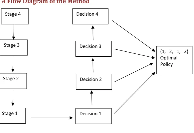
A Flow Diagram of the Method

3. Presentation and Analysis of Data

3.1. Presentation of Data

The data to be presented here are:

1) Cadres of lecturers and level of statistics courses, see Table 1.

2) Cadres of lecturers and credit hours per statistics courses, see Table 2.

3.2. Analysis of Data

The standard form of dynamic programming when the final state is fixed and initial state is free is given by

(

)

( )

(

)

n n n x n i n n n

f s x =opt R x + f∗+ s −x  (7)

where xiare the stages and Siare the states, i=1, 2,,n.

In this section, we analyze the data presented in Tables 3-7.

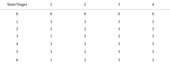
1) We represent different cadres of lecturers as “State” and level of courses as “Stages”. Here, we have six states and four stages. Zeroes in the second row represent the origin where no allocation has been made. This is represented in

Table 3.

2) Table 4 is derived from the state and last column of Stage 4 from Table 3, since the last stage is fixed.

Stage 4

Stage 3

Stage 2

Stage 1 Decision 1

Decision 2 Decision 3 Decision 4

DOI: 10.4236/ojop.2017.64012 181 Open Journal of Optimization

Table 1. Cadres of lecturers and level of STA courses.

Cadre of lecturers 200 Level 300 Level 400 Level 500 Level Professors 1 STA 211 STA 301 STA 411 STA 501 Readers 2 STA 221 STA 321 STA 421 STA 511 Senior lecturers 3 STA 223 STA 331 STA 431 STA 513 Lecturer 1 4 STA 212 STA 312 STA 433 STA 502 Lecturer 11 5 STA 222 STA 336 STA 435 STA 512 Ass. lecturer 6 STA 224 STA 342 STA 451 STA 514

Source: Department of Statistics, FUTO (2017).

Table 2. Cadres of lecturers and credit hours per STA courses.

Cadre of lecturers 200 Level 1 300 Level 2 400 Level 3 500 Level 4 Professors 1 3 3 3 3

Readers 2 3 3 3 3 Senior lecturers 3 1 3 2 3 Lecturer 1 4 3 3 3 3 Lecturer 11 5 3 3 3 3 Ass. lecturer 6 1 3 3 3

Table 3. State and stages.

State/Stages 1 2 3 4

0 0 0 0 0

1 3 3 3 3

2 3 3 3 3

3 1 3 2 3

4 3 3 3 3

5 3 3 3 3

6 1 3 3 3

Table 4. Stage 1 of the problem.

S4 f4

∗

4 X∗

0 0 0

1 3 1

2 3 2

3 3 3

4 3 4

5 3 5

DOI: 10.4236/ojop.2017.64012 182 Open Journal of Optimization

Table 5. Stage 2 of the problem.

S3/X3 0 1 2 3 4 5 6 f3

∗

3 X∗

0 0 0 0

1 3 3 3 0 or 1

2 3 6 3 6 1

3 3 6 6 2 6 1 or 2

4 3 6 6 5 3 6 1 or 2

5 3 6 6 5 6 3 6 1, 2 or 4

6 3 6 6 5 6 6 3 6 1, 2, 4 or 5

Table 6. Stage 3 of the problem.

S2/X2 0 1 2 3 4 5 6 f2

∗

2 X∗

0 0 0 0

1 3 3 3 0 or 1 2 6 6 3 6 0 or 1 3 6 9 6 3 9 1 4 6 9 9 6 3 9 1 or 2 5 6 9 9 9 6 3 9 1, 2 or 3 6 6 9 9 9 9 6 3 9 1, 2, 3 or 4

Table 7. Stage 4 (final stage) of the problem.

S1/X1 0 1 2 3 4 5 6 f1

∗

1 X∗

0 0 0 0

1 3 3 3 0 or 1 2 6 6 3 6 0 or 1 3 9 9 6 1 9 0 or 1 4 9 9 9 4 3 9 0, 1 or 2 5 9 12 12 7 6 3 12 1, or 2 6 9 12 12 10 9 6 1 12 1 or 2

3) Tables 5-7 are obtained recursively from Equation (7) using Table 4 as the first stage.

Since the final stage was fixed, we obtain Table 4 from the first and last

col-umn of Table 3 above. The optimal value X4

∗ _{correspond to the values in the}

column of S4.

Applying the formula in Equation (7) and using Table 4 as a starting point,

we obtain Tables 5-7 below. See Appendices 1-3 for the computation of these

Tables respectively.

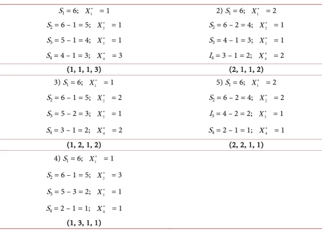
In Table 8, we calculate the optimal course allocations starting from Table 7. This is calculated by taking the various combinations from the last value of state

(S1) as 6 and X1

∗ _{= 1. And we do the needed computations as shown in Table 8}

DOI: 10.4236/ojop.2017.64012 183 Open Journal of Optimization

Table 8. Optimal allocations.

S1 = 6; X1

∗ _{= 1 2) S}

1 = 6; X1

∗ _{= 2}

S2 = 6 – 1 = 5; X2

∗ _{= 1} S

2 = 6 – 2 = 4; X2

∗ _{= 1}

S3 = 5 – 1 = 4; X3

∗ _{= 1 S}

3 = 4 – 1 = 3; X3

∗ _{= 1}

S4 = 4 – 1 = 3; X4

∗ _{= 3 I}

4 = 3 – 1 = 2; X4

∗ _{= 2}

(1, 1, 1, 3) (2, 1, 1, 2) 3) S1 = 6; X1

∗ _{= 1} 5) S

1 = 6; X1

∗ _{= 2}

S2 = 6 – 1 = 5; X2

∗ _{= 2 S}

2 = 6 – 2 = 4; X2

∗ _{= 2}

S3 = 5 – 2 = 3; X3

∗ _{= 1 I}

3 = 4 – 2 = 2; X3

∗ _{= 1}

S4 = 3 – 1 = 2; X4

∗ _{= 2 S}

4 = 2 – 1 = 1; X4

∗ _{= 1}

(1, 2, 1, 2) (2, 2, 1, 1) 4) S1 = 6; X1

∗ _{= 1}

S2 = 6 – 1 = 5; X2

∗ _{= 3}

S3 = 5 – 3 = 2; X3

∗ _{= 1}

S4 = 2 – 1 = 1; X4

∗ _{= 1}

(1, 3, 1, 1)

Thus, the allocation of courses to lectures according to Table 8 above will

yield estimated optimum credit hours of 12 for each lecturer per semester. See

the last value in f1

∗ _{of Table 7.}

4. Interpretation of Results

Calculations in Section 3.2 are presented in Appendices 1-3. Hence, the optimal

allocation policy of (1, 1, 1, 3) in Table 8 means the allocation of one Statistics

course to each lecturer in each cadre in second, third, fourth year and three courses to each cadre of lecturer in the fifth (final) year will yield optimal credit hour of 12 for each lecturer per semester.

(2, 1, 1, 2) in Table 8 means the allocation of two Statistics courses to each

lecturer in each cadre in second year, one course each in third and fourth year and two courses to each cadre of lecturer in the fifth (final) year will yield op-timal credit hour of 12 for each lecturer per semester.

(1, 2, 1, 2) in Table 8 means the allocation of one Statistics course to each

lec-turer in each cadre in second year, two courses each to each leclec-turer in third year, one course to each lecturer in fourth year and two courses to each cadre of lecturer in the fifth (final) year will yield optimal credit hour of 12 for each lec-turer per semester.

(1, 3, 1, 1) in Table 8 means the allocation of one statistics course to each

lec-turer in each cadre in second year, three courses each to each leclec-turer in third year, one course to each lecturer in fourth year and one course to each lecturer in each cadre in the fifth (final) year will yield optimal credit hour of 12 for each lecturer per semester.

(2, 2, 1, 1) in Table 8 means the allocation of two Statistics courses to each

DOI: 10.4236/ojop.2017.64012 184 Open Journal of Optimization

fifth year courses to each lecturer in each cadre will yield optimal credit hour of 12 for each lecturer per semester.

5. Conclusion

In this paper, dynamic programming was applied in allocating courses to lectur-ers in the Nigerian univlectur-ersities, using the Department of Statistics, Federal Uni-versity of Technology, Owerri, Imo State as a case study. An optimal 12 credit hours was obtained for each lecturer in each cadre for the semester. Among all the optimal allocations policies presented in section 4, the best optimal alloca-tion is achieved at the point (1, 2, 1, 2). This means that each lecturer should be assigned at most one course in both harmattan and rain semester of second year and one course in harmattan semester of fourth year when fewer number of Sta-tistics courses are offered due to introduction of StaSta-tistics courses to second year students and also due to six-month industrial training by the fourth year stu-dents in the rain semester. On the other hand, lecturers should be allocated two courses each in the third and fifth year rain and harmattan semesters, when all the students are back for their normal academic session. Allocation of courses in this order will yield an optimal credit hour of 12 per lecturer per semester. This is highly reasonable as opposed to the use of rule of thumb which overload some lecturers with more courses and under load others with fewer courses.

References

[1] Rao, S.S. (2009) Engineering Optimization: Theory and Practice. 4th Edition, John Wiley & Sons, Inc., Canada.

[2] Esogbue, A.O. and Marks, B.R. (1974) Non-Serial Dynamic Programming: A Sur-vey. Journal of the Operational Research Society, 25, 253-265.

[3] Adelson, R.M., Norman, J.M. and Laporte, G. (1976) A Dynamic Programming Formulation with Diverse Applications. Journal of the Operational Research Socie-ty, 27, 119-121.

[4] Smith, P. (1989) Dynamic Programming in Action. Journal of the Operational

Re-search Society, 40, 779-787.

[5] Wong, P.J. (1970) A New Decomposition Procedure for Dynamic Programming.

Operations Research, 18, 119-131.https://doi.org/10.1287/opre.18.1.119

[6] Howard, R.A. (1966) Dynamic Programming. Operations Research, 12, 317-348.

https://doi.org/10.1287/mnsc.12.5.317

[7] Moores, B. (1986) Dynamic Programming in Transformer Design. Journal of the

Operational Research Society, 37, 967-969.

[8] Jensen, R.E. (1969) A Dynamic Programming Algorithm for Cluster Analysis.

Op-erations Research, 17, 1034-1057.https://doi.org/10.1287/opre.17.6.1034

[9] Nemhauser, G.L. and Ullmann, Z. (1969) Discrete Dynamic Programming and Capital Allocation. Operations Research, 15, 494-505.

DOI: 10.4236/ojop.2017.64012 185 Open Journal of Optimization

Appendices

Computations of Tables 5-7

In these appendices, we show how Tables 5-7 were computed from Equation

(7). The values of current state and stages were substituted while the previous stage forms the starting point in the current stage. This recursive relationship continues until the final stage is obtained.

Appendix 1. Computation of Stage 2 presented in Table 5.

For n = 3, we have n(3,0): = R3(0) + f4

∗_{(3) = 0 + 3 = 3}

f3(S3,X3) = R3(X3) + f4

∗_(S

3 − X3) n(3,1): = R3(1) + f4

∗_{(2) = 3 + 3 = 6}

n(0,0): f3(0,0) = R3(0) + f4

∗_{(0 − 0) n(3,2): = R}

3(2) + f4

∗_{(1) = 3 + 3 = 6}

= R3(0) + f4

∗_{(0) = 0 n (3,3): = R}

3(3) +f4

∗_{(0) = 2 + 0 = 2}

n(1,0): f3(1, 0) = R3(0) + f4

∗_{(1 − 0) n(4,0): = R}

3(0) + f4

∗_{(4) = 0 + 3 = 3}

= R3 (0) + f4

∗_{(1) = 0 + 3 = 3 n(4,1): = R}

3(1) + f4

∗_{(3) = 3 + 3 = 6}

n(1,1): f3(1,1) = R3(1) + f4

∗_{(0) = 3 + 0 = 3 n(4,2): = R}

3(2) +f4

∗_{(2) = 3 + 3 = 6}

n(1,1): f3(1,1) = R3(1) + f4

∗_{(0) = 3 + 0 = 3 n(4,3): = R}

3(3) + f4

∗_{(1) = 2+3 = 5}

n (2,0): = R3(0) + f4

∗_{(2) = 0 + 3 = 3 n(4,4): = R}

3(4) + f4

∗_{(0) = 3 + 0 = 3}

n(2,1): = R3(1) + f4

∗_{(1) = 3 + 3 = 6 n(5,1): = R}

3(1) + f4

∗_{(4) = 3 + 3 = 6}

n(2,2): = R3(2) + f4

∗_{(0) = 3 + 0 = 3} n (5,2): = R

3(2) + f4

∗_{(3) = 3 + 3 = 6}

n(5,0): = R3(0) + f4

∗_{(5) = 0 + 3 = 3 n(5,3): = R}

3(3) + f4

∗_{(2) = 2 + 3 = 5}

n(6,0): = R3(0) + f4

∗_{(6) = 3 n(5,4): = R}

3(4) + f4

∗_{(1) = 3 + 3 = 6}

n(6,1): = R3(1) + f4

∗_{(5) = 6} n(5,5): = R

3(5) + f4

∗_{(0) = 3 + 0 = 3}

n(6,2): = R3(2) + f4

∗_{(4) = 6}

n(6,3): = R3(3) + f4

∗_{(3) = 5}

n(6,4): = R3(4) + f4

∗_{(2) = 6}

n(6,5): = R3(5) + f4

∗_{(1) = 6 n (6,6): = R}

3(6) + f4

∗_{(0) = 3}

Appendix 2. Computation of Stage 3 presented in Table 6.

For n = 2, we have n(4,3) = R2(3) + f3

∗_{(1) = 3 + 3 = 6}

f2(S2,X2) = R2(X0) + f3

∗_(S

2 – X2) n(4,4) = R2(4) + f3

∗_{(0) = 3 + 0 = 3}

f2(0, 0) = R2(0) + f3

∗_{(0) = 0 n(5,0) = R}

2(0) + f3

∗_{(5) = 0 + 6 = 6}

n(1,0) = R2(0) + f3

∗_{(1) = 3 n(5,1) = R}

2(1) + f3

∗_{(4) = 3 + 6 = 9}

n(1,1) = R2(1) + f3

∗_{(0) = 3 n(5,2) = R}

2(2) + f3

∗_{(3) = 3 + 6 = 9}

n(2,0) = R2(0) + f3

∗_{(2) = 6 n(5,3) = R}

2(3) + f3

∗_{(2) = 3 + 6 = 9}

n(2,1) = R2(1) + f3

∗_{(1) = 6 n(5,4) = R}

2(4) + f3

∗_{(1) = 3 + 3 = 6}

n(2,2) = R2(2) + f3

∗_{(0) = 3 n(5,5) = R2(5) +}

3

f∗(0) = 3 + 0 = 3

n(3,0) = R2(0) + f3

∗_{(3) = 6 n(6,0) = R}

2(0) +f3

DOI: 10.4236/ojop.2017.64012 186 Open Journal of Optimization Continued

n(3,1) = R2(1) + f3

∗_{(2) = 3 + 6 = 9 n(6,1) = R}

2(1) + f3

∗_{(5) = 3 + 6 = 9}

n(3,2) = R2(2) + f3

∗_{(1) = 3 + 3 = 6 n(6,2) = R}

2(2) + f3

∗_{(4) = 3 + 6 = 9}

n(3,3) = R2(3) + f3

∗_{(0) = 3 + 0 = 3 n(6,3) = R}

2(3) + f3

∗_{(3) = 3 + 6 = 9}

n (4, 0) = R2(0) + f3

∗_{(4) = 0 + 3 = 3 n (6, 4) = R}

2(4) + f3

∗_{(2) = 3 + 6 = 9}

n (4, 2) = R2(2) + f3

∗_{(2) = 3 + 6 = 9} n (6, 5) = R

2(5) + f3

∗_{(1) = 3 + 3 = 6}

n (6, 6) = R2(6) + f3

∗_{(0) = 3 + 0 = 3}

Appendix 3. Computation of Stage 4 presented in Table 7.

For n = 1, we have n(4,3) = R1(3) + f2

∗_{(1) = 1 + 3 = 4}

f1(S1,X1) = R1(X1) + f2

∗_(S

1 – X1) n(4,4) = R1(4) + f2

∗_{(0) = 3 + 0 = 3}

f1(0,0) = R1(0) + f2

∗_{(0) = 0 n(5,0) = R}

1(0) + f2

∗_{(5) = 9}

n(1,0) = R1(0) + f2

∗_{(1) = 3 n(5,1) = R}

1(1) + f2

∗_{(4) = 3 + 9 = 12}

n(1,1) = R1(1) + f2

∗_{(0) = 3 + 0 = 3 n(5, 2) = R}

1(2) + f2

∗_{(3) = 3 + 9 = 12}

n(2,0) = R1(1) + f2

∗_{(2) = 6 n(5, 3) = R}

1(3) + f2

∗_{(2) = 1 + 6 = 7}

n(2,1) = R1(1) +f2

∗_{(1) = 3 + 3 = 6 n(5, 4) = R}

1(4) + f2

∗_{(1) = 3 + 3 = 6}

n (2, 2) = R1(2) +f2

∗_{(0) = 3 + 0 = 3 n(5, 5) = R}

1(5) + f2

∗_{(0) = 3 + 0 = 3}

n (3, 0) = R1(0) + f2

∗_{(3) = 9 n(6,0) = R}

1(0) + f2

∗_{(6) = 9}

n(3,1) = R1(1) +f2

∗_{(2) = 3 + 6 =9 n(6,1) = R}

1(1) +f2

∗_{(5) = 3 + 9 = 12}

n(3,2) = R1(2) + f2

∗_{(1) = 3 + 3 = 9 n(6, 2) = R}

1(2) + f2

∗_{(4) = 3 + 9 = 12}

n(3,3) = R1(3) + f2

∗_{(0) = 1 n(6,3) = R}

1(3) + f2

∗_{(3) = 1 + 9 = 10}

n(4,0) = R1(0) + f2

∗_{(4) = 9 n (6, 4) = R}

1(4) + f2

∗_{(2) = 3 + 9 = 9}

n(4,1) = R1(1) + f2

∗_{(3) = 3 + 6 = 9 n(6,5) = R}

1(5) + f2

∗_{(1) = 3 + 3 = 6}

n(4,2) = R1(2) + f2

∗_{(2) = 3 + 6 = 9 n(6,6) = R}

1(6) + f2