Evaluate the Affected Factors on Student's Mathematics Performance in Rural Areas by Estimating an Education Production Function : As a Case Study of Passara Educational Zone, Sri Lanka

(1)

EVALUATE

THE

AFFECTED

FACTORS

ON

STUDENTS’

MATHEMATICS

PERFORMANCE

IN

RURAL

AREAS

BY

ESTIMATING

AN

EDUCATION

PRODUCTION

FUNCTION:

AS

A

CASE

STUDY

OF

PASSARA

EDUCATIONAL

ZONE,

SRI

LANKA

E.V.D.Dilhani

Department of Economics, University of Ruhuna, Matara, Sri Lanka

ABSTRACT

Student’s ability in mathematics is an important component regarding with their cognitive achievement. There is a general assumption among educationists that mathematics can develop people’s logical and analytical thinking. G.C.E. ordinary level exam in the Sri Lanka is an important stage to make a clear picture of student’s mathematical ability in Sri Lanka. Unfortunately, student’s results regarding with mathematics is so week in Sri Lanka. This study aimed to find the affected factors on student’s mathematics performance. This study has done as a case study in Passara educational zone, Sri Lanka. Multiple liner regression analysis used as the estimation technique. This study finalized that tuition class hours, education level of the most helpful person for student’s education at home and student teacher ratio at class room in school make significant effect on student’s mathematics performance. So, it’s clear that to improve the results regarding with mathematics in considering area should improve and provide the educational sources for students.

KEYWORDS

Economics of Education, Education Production Function, Multiple Linear Regression, Mathematics, Educational inputs.

1. INTRODUCTION

The ability in mathematics improve the human’s cognitive rational skills. It effect on human’s career life and day to day life. Education policy makers pay their attention on Mathematics because of the extraordinary uses of the score in mathematics as a measure of education performance. Because of that the results of mathematics has come to an important condition relevant to the other subjects. As well as like in job strategies also.

Dr. Fan Chang once said that ‘in mathematics whatever you learn is yours and your build up one step at a time. It’s not like a real-time game of winning and losing. You win if you benefit from the power, rigor and beauty of mathematics’. There is a general assumption among the researchers that everyone should be required to take some level of mathematics. Mathematics is one of major thing can only help people to think logically and analytically.

(2)

International Journal of Education (IJE) Vol.5, No.2, June 2017

Data source: Department of examination, 2015

So, this research aimed to find the

evaluate this problem the most appropriate area should be a weak area.

To derive that mater graphs two figure the variation of results in

Badulla district is in poor level in mathematics performance of the students.

Data source: Department of examination, 2015 0

20 40 60

P

er

se

n

ta

g

e

of

c

an

d

id

at

es

G.C.E. O/L Mathematics results in four

Journal of Education (IJE) Vol.5, No.2, June 2017 Figure No. 01

So, this research aimed to find the efforts which effect on students mathematics education. To evaluate this problem the most appropriate area should be a weak area.

Figure No. 02

To derive that mater graphs two figure the variation of results in some districts. So comparatively Badulla district is in poor level in mathematics performance of the students.

Figure No. 03

A B C S W

Grade

G.C.E. O/L Mathematics results in four districts-2015

Colombo Kandy Matara Badulla

on students mathematics education. To

(3)

Figure 3 show that the difference in mathematical performance among the educational zones in Badulla district. There are five educational zonal areas in Badulla district. But passara education zone lowest results in A , B, C and it is in high level in weak strategies. So this study aims to identify the factors relative with student’s poor performance in considering area.

Student’s education performance consider as the education out come and factors which affect to the students educational outcome can mention as the educational input variables. In education researches there is a common term called Education Production Function (EPF). Education production function is a model to show the relationship between education input output relationship. Ransing he has cited as ‘A systematic investigation of the relationship between school input and student performances is condensed in the education production function’. Education production function concept has initiated from relatively economics of education subject. Theoretically, economics of education narrates the conduction of education towards economic development. The concept of Education Production Function (EPF) introduced “Coleman Report” of 1966. It made a rational change in the estimations regarding with education.The estimation of this study is based the multiple linear regression model. The analysis is based on primary and secondary both type of data. The review of relevant literature, methodology, analysis and conclusions beyond.

1.1Research Problem

The research problem of the study is to identify the affected factors on student’s weak mathematical performance in rural area. The primary data relevant to the educational inputs and output have gathered from the students who in passara education zone by using questioner.

1.2 Review of the relevant literature

There are number of researches in education field relevant to the estimation of education production function. But here there are some expiations about some selected studies relevant with mathematics and the multiple linear regression estimation technique.

Lamdin (2001) has studied about the evidence of student attendance as an independent variable in education production functions. He specified the student’s attendance as an independent variable of his study. The dependent variable of the study was student performance on the California achievement test (CAT) in the spring of 1989. The cat has reading portion and a mathematics portion. The independent variables of the study are under main two sectors. First one is student sector. Student sector variables are innate student ability, parental background, and socioeconomic states. School sector variables are teacher/pupil ratio, expenditure per pupil, amount of education experience of the teacher. There was single output in this study. So, he used the regression model to interpret the results. The conclusions of the study were the influence of attendance on student performance may or may not differ substantially by school or teacher. This is an important and potentially illuminating issue to address. In any case, analysis are well advised to further document the robustness of the attendance performance relationship with other data because the finding reported here should not be viewed as the last word on the matter.

(4)

percentage of economically disadvantaged students. The study used multivariate methods to examine and explain the relationships between three educational inputs and two outputs using a data matrix from 71 highs schools in six schools districts in the metropolitan Atlanta, Georgia area. Combinations for multivariate analysis of variance (Manova), Canonical correlation analysis (CCA), and multivariate regression analysis (MRA) were used in the analysis of the data. The concluded that money matters as a determinant of student achievement when the economic states of students is considered as an integral part of the educational output mix.

Brempong and Gyapong (1991) have done a research regarding with education production function. They have used the cross section data in 175 school districts with a population of 1000 or more in the state of Michigan. The dependent variable of the study is the education output of the students. They used the score in mathematics and score in English to measure the education outcome of the children. The independent variables of the study are school resources, student’s characteristics and social economic characteristics (SEC) of the students. The canonical regression analysis was used to investigate the effects of regarding inputs in the production of high school education. Finally they have concluded that education of parents is the only variable that can be used as a proxy for all SEC without miss specifying the education production function.

Ismail and Cheng (1997) have study about the education production in Malaysia. This study used data from national sources and third international mathematics and science study carried out in 1999. The sample of the study was selected using the simple random sampling. There were 150 schools in Malaysia and the population of the study was 5,715. After excluding missing values and making necessary correlations, data from 131 schools and 4854 students are used for this study. The dependent variables of the study are the test score in mathematics and science.

The independent variables of the study are pupil non-teaching recurrent expenditure, pupil teacher ratio, teachers with more than five years’ experience, yearly school hours spent on instruction, student with at least medium level in home educational resources index, students with at least medium level in out of school study index and number of female students in class. Canonical regression analysis uses as the methodology of the study.

The analysis of the tests demonstrates the significant effects of home education resources on the Malaysian school’s mathematics and science achievement. Furthermore, pupil teacher ratio appears to be most productive input among the educational inputs conceded. Last but not least, it finds that instructional hours can be offset the low level of out of school study time.

Ekrem, Selma and Adem (2010) explored the factors effects on student’s mathematical achievement in Grade 6th, 7th and 8th in secondary schools. The explanatory variables selected as type of school, family income, studying time and students’ attitude towards mathematics and attendance to private courses have been investigated. Descriptive statistics and chi-square analysis involved to the analysis.

The results of study showed that type of school, family income, studying time, students’ attitude towards mathematics and attendance to private courses had statistically significant effects on students’’ mathematics achievement.

(5)

2. METHODOLOGY

Hanushek (1986, as cited by Ranasinghe) identified three major drawbacks in educational production process. First one is the absence of a proper theoretical framework to justify the pressured production process. Second and third were the difficulties associated with identifying input and output of the education production process. An estimation of education production function should consist with some mapping rules and it must satisfy several mathematical properties (Ranasinghe).

1. It must be a single output.

2. It has continuous first and second order partial derivatives.

3. The first derivative is positive and second order partial derivatives is negative by assumption.

The estimation technique of the study is multiple linear regression. The model of the EDF is assuming Cobb-Douglas type production function. The Cobb-Douglas production function derive on basic two concepts such as cost reduction concept and profit maximization concept. But in education production function analysis those have ignored.As well as to estimate nonlinear relationship by using linear technique it’s a must to convert data to ‘Ln’ form. General model of the multiple linear regression is as follow,

Yi=ß0+ß1Xi1+ß2Xi2+…+ßpXip+ei

i = observational unit from which the observations on Y. p = independent variable were taken.

The model of the education production function regression in mathematics based on multiple linear as follow,

MATSC=β0+ β1 GNDR+ β2 FRTM+ β3 SLTM +β4 ATEND +β5 TUTIN +β6 STUHR +β7

MOTED+β8 FATED+β9 FYHLED+β10 INCM+β11 HOMER +β12 PEER+β13 STR +u

Secondary data have gathered from the evaluation reports have been published by research and development branch of department of examinations. Primary data gathered from the survey in Passara education zone done by the author. There were 203 units in the sample and two stage cluster sampling has used to select the sample units.

The list of variables is as follow,

Educational Outcome (Dependent Variable)

• MATSC - Test score in Mathematics

Educational inputs (Independent Variables)

• GNDR - Gender

• FRTM -Free hours per day

• SLTM -Sleeping hours per day

• ATEND -Number of school present days in considering year

• TUTIN -Number of tuition class hours per week for mathematics

• STUHR -Number of self-study hours per week in mathematics

• MOTED - Mother’s education level

• FATED - Father’s education level

• FYHLED - Education level of the most helpful person for

the student’s education at the home

• INCM -Gross month salary of household

• HOMER - Ability in uses of educational resources at home

• PEER -Education level of the buddy

(6)

There are ten assumptions relative with the multiple linear regression (Gujarati, 2004).

1. Linear regression model. The regression model is linear in the parameters. As shown in

follow.

Yi=ß1+ß2Xi+ui

2. X values are fixed in repeated sampling. Values taken by the regressor X are considered

fixed in repeated samples. More technically. X is assumed to be nonstochastic.

3. Zero mean values of disturbance ui. Given the value of X, the mean, or expected, value

of the random disturbance term ui, is zero technically, the conditional mean value of ui is

zero symbolically, we have

E(ui | Xi)=0

4. Homoscedasticity or equal variance of ui. Given the value of x, the variance of ui is the

same for all observations. That is, the conditional variances. That is, the conditional variances of ui are identical. symbolically we have,

Var (ui|Xi) = E[(ui-E(ui|Xi)]2

= E(ui|Xi) because of assumption 3

=σ2

Where Var stands for variance.

5. No autocorrelation between the disturbances. Given any two X values, Xi and Xj (i ≠

j), the correlation between any two ui and uj (i ≠ j) is zero. Symbolically,

Cov ( ui, uj | Xi, Xj) = E ([ui-E(ui)]|Xi){[uj-E(uj)] | Xj}

= E (ui | xi) (uj | xj)

= 0

Where i and j are two different observations and where cov means covariance.

6. Zero covariance between ui and xi, or E(ui xi)=0. Formally,

Cov(ui,xi) =E[ui-E(vi)][xi-E(xi)]

=E[ui(xi-E(xi))] since E(ui)=0

=E (uixi)-E(xi)E(ui) Since E(xi) is nonstochastic

=E( ui Xi) Since E(ui)=0

=0 by assumption

7. The number of observations n must be greater than the number of parameters to be

estimated. Alternatively, the number of observations n must be greater than the number of explanatory variables.

8. Variability in X values. The x values in a given sample must not all be the same.

Technically, Var (X1) must be a finite positive number.

9. The regression model is correctly specified alternatively, there is no specification bias or error in the model used in empirical analysis.

10.There is no perfect multicollinearity. That is, there are no perfect linear relationships among the explanatory variables.

(7)

3. RESULTS

AND

FINDINGS

The statistical analysis of this study con

regression estimation with all variables. Second one is the step wise regression estimation. Table No 01 consist with the results of estimation of all variabl

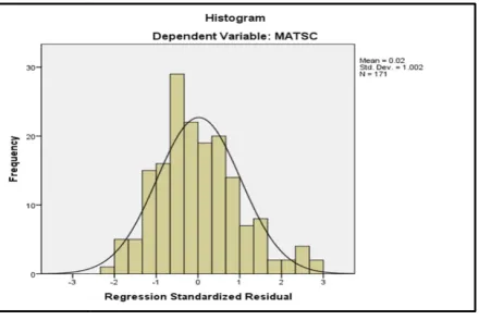
[image:7.612.199.419.208.355.2]

wise regression results. The assumption Randomness of the dependent variable

Figure No 04: Histrogam of dependent variable

Other assumptions can check by using

01 consist with the multiple linear regression results with all variables. The R value derive the correlation between independent variables and

is greater than 0.5 that means there is a positive strong relationship between students’ mathematics score and independent variables. The R

should distribute between 0 and 1. Here it is 0.377. That means the model predictable level. The Durbin Watson results also same to

an autocorrelation error in the estimation.

could interpret table 01 results figure the significant variables on students’ mathematics education. Because the model was significant from the ANOVA test.

model was significant. Then the homoscedasticity also was the estimation. There is no any pattern in the graph so it means there is no heteroscedasticity error in the model.

there were three significant factors

participation to the tuition class, scarcity of educational resources at home in considering area and student teacher ratio. But it wasn’t possible to interpret the coefficient relevant to those variables. Because of the weakness of the model fit.

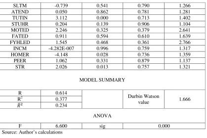
Table No 01: Results of Multiple linear regression analysis with all variables.

Model

coefficient

Constant 23.479

GNDR 3.723

FRTM 1.016

FINDINGS

of this study consist with two parts. First one was the multiple linear regression estimation with all variables. Second one is the step wise regression estimation. Table No 01 consist with the results of estimation of all variables and Table no 02 consist with the step he assumptions of the estimation have checked with the estimations. Randomness of the dependent variable

igure No 04: Histrogam of dependent variable

Source: Author’s estimations

assumptions can check by using the results regarding with the table No 01 and 02.

multiple linear regression results with all variables. The R value derive the correlation between independent variables and dependent variables. It was a positive value and it is greater than 0.5 that means there is a positive strong relationship between students’ mathematics score and independent variables. The R2 value is the coefficient of determination. It

between 0 and 1. Here it is 0.377. That means the model coefficients predictable level. The Durbin Watson results also same to above prediction. That figures there is an autocorrelation error in the estimation. Even if the model fit wasn’t sufficient the coefficients could interpret table 01 results figure the significant variables on students’ mathematics Because the model was significant from the ANOVA test. That means the overall was significant. Then the homoscedasticity also was the estimation. There is no any pattern in the graph so it means there is no heteroscedasticity error in the model. Table no 01

factors on students’ mathematics performance such at Students’ class, scarcity of educational resources at home in considering area and student teacher ratio. But it wasn’t possible to interpret the coefficient relevant to those variables.

ss of the model fit.

Table No 01: Results of Multiple linear regression analysis with all variables.

COEFFICIENTS

coefficient Sig Collinearity statistics

Tolerance 0.438

0.237 0.718

0.396 0.647

the multiple linear regression estimation with all variables. Second one is the step wise regression estimation. Table es and Table no 02 consist with the step s of the estimation have checked with the estimations.

the results regarding with the table No 01 and 02. Table no multiple linear regression results with all variables. The R value derive the dependent variables. It was a positive value and it is greater than 0.5 that means there is a positive strong relationship between students’ value is the coefficient of determination. It coefficients not in figures there is the coefficients could interpret table 01 results figure the significant variables on students’ mathematics That means the overall was significant. Then the homoscedasticity also was the estimation. There is no any pattern Table no 01 derive that erformance such at Students’ class, scarcity of educational resources at home in considering area and student teacher ratio. But it wasn’t possible to interpret the coefficient relevant to those variables.

Collinearity statistics VIF

(8)

SLTM -0.739 0.541 0.790 1.266

ATEND 0.050 0.862 0.781 1.281

TUTIN 3.112 0.000 0.713 1.402

STUHR 0.204 0.139 0.906 1.104

MOTED 2.246 0.325 0.379 2.641

FATED 0.911 0.594 0.610 1.639

FYHLED 1.545 0.468 0.361 2.766

INCM -4.282E-007 0.996 0.759 1.317

HOMER -4.148 0.028 0.736 1.359

PEER 1.062 0.331 0.879 1.137

STR 2.026 0.013 0.757 1.321

MODEL SUMMARY

R 0.614

Durbin Watson

value 1.666

R2 0.377

0.234

ANOVA

F 6.600 sig 0.000

[image:8.612.102.521.75.354.2]

Source: Author’s calculations

Figure No 05

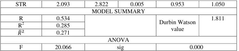
The step wise estimation relevant to the education production function estimation in Mathematics

was in table no 02. That also weak in R2 but Strong in R as well as Durbin wotsan value. Here

there is no any multicolliniarity error or heterosdacasticity error or autocorrelation error (According to the Durbin wotsan value, tolerance value/ VIF value and Figure 06).

Table No 02: Results of step wise multiple linear regression estimation. COEFFICIENTS

Model coefficient t Sig Collinearity statistics

Tolerance VIF

Constant 18.534 4.369 0.000

TUTIN 2.926 4.659 0.000 0.895 1.117

[image:8.612.200.407.424.550.2]

(9)

STR 2.093 2.822 0.005 0.953 1.050 MODEL SUMMARY

R 0.534

Durbin Watson value

1.811

R2 0.285

0.271

ANOVA

F 20.066 sig 0.000

[image:9.612.110.525.79.168.2]

Figure No 06 Source: Author’s calculations

The step wise multiple linear regression analysis prove that it is a predictable estimation as well as there were three significant variables there those are students’ participation to the tuition class and student teacher ratio at school and the education level of most helpful person at home effect on students’ mathematics performance positively.

4. CONCLUSIONS

AND

RECOMMENDATIONS

This study gives a clear idea that students’ tuition class make a significant effect on students’ mathematics performance. As well as education level of the most helpful person at home and student teacher ratio at the school also make positive effect on student mathematical performance. Comparatively education level of the most helpful person at home effected on students’ mathematic education than tuition class and the student teacher ratio. So, it’s clear that the education level of student family also should be considerable situation. The study area was a rural area the people who live in that area not more focusing on education like other areas in Sri Lanka. So it’s important to improve the literacy level in mathematics in all people in considering area as well as country. Because it improve people’s critical thinking ability. That effect to make the human capital of a nation. So, this is an important point to policy makers and rules to pay their attention.

ACKNOWLEDGEMENTS

(10)

REFERENCES

1. Agunloye O. Olajde, Sielike C. Catherine, Jnik Stephen Ole, 2005, A multivariate analysis of education productivity in urban Georgia high school, Georgia, http://coefaculty.valdosta.edu/lschmert/.../multivariate-finalbyLS2007.pdf.

2. Brempony K.G. & Gyapoma A,1990, ‘Characteristics of educational production functions: An application of canonical regression analysis’, Economics of education review,vo10, No 1, p 7-19,Great Britain.

3. Gujarati N. D., 2004, Basic Econometrics, fourth edition, The McGraw Hill Company.

4. Ismail N.A & Cheng A.G, 1991, ‘The relationship between cognitive performance and critical thinking abilities among selected agricultural education students’, Journal of agricultural education.

5. Lamdin J. Douglas, 2001, Evidence of student attendance as an independent variable in education production function, the journal of educational research, January/February 1996, Vol 89, no 3.

6. Ranasinghe A, A pearl of great price: the free education system of Sri Lanka, faculty of economics and business, http://dare.uva.nl/document/473462.

Author

E.V.D.Dilhani is a Bachelor of Arts (Special) in Social Statistics with Second Class (Upper Division) Honors from University of Ruhuna, Sri Lanka. Currently she works as the temporary assistant lecturer in Social Statistics in Department of Economics, University of Ruhuna. As well as she has qualified in Diploma in Human resource management. She would rather interesting in educational sector in her research studies.

APPENDIXES

Appendixes no 01-SPSS output of multiple linear regression estimation with all variables

(11)