Applications of SIFT-MS to the
Environment and Petroleum Exploration
A thesis presented for the degree
Of
Master of Science in
Chemistry
By
Majed Mohammed Alghamdi
Title page
Table of contents... iii
Acknowledgement……….. viii
Abstract……….. ix
List of Figures... x
List of Tables……….. xv
Chapter 1: Introduction to SIFT-MS methodology 1. Introduction……….. 1
1.1Ion-molecule reactions……….……….. 1
1.2Applications of ion-molecule reactions……..……… 2
1.3SIFT-MS……… 3
1.3.1Overview……… 3
1.3.2SIFT-MS Instrument………... 4
1.3.2.1Ion source region………... 5
1.3.2.2Ion reaction region……….……… 6
1.3.2.3Ion detection region………... 7
1.3.2.4Quadrupole mass filter………... 8
1.3.2.5Einzel lenses……….. 10
1.3.2.6Multiplier………... 10
1.3.2.7Pumps………....…… 11
1.3.3How SIFT-MS works……… 14
1.3.4Important points in SIFT-MS technique………... 16
1.3.5Ion molecular reaction in SIFT-MS……….. 18
1.3.5.1H3O+ reactions………. ……. 18
1.3.5.2NO+ reactions………. 19
1.3.5.3O2+ reactions……….. 20
1.3.6Kinetic and rate coefficient……….……... 21
1.3.7.1Mass scan mode………. 23
1.3.7.2SIM scan mode……….. 24
Chapter 2: Preliminary preparations and experiments 1. Introduction ………..…... 25
2. Preliminary work………....………..………... 25
2.1 Instrument calibration……….. 25
2.1.1 Instrumental Calibration Factor (ICF)………....……..… 25
i. The Constant Cumulative Count (3C method)…………....……... 26
ii. New calibrated cylinder method……….. 27
2.1.2 Quadrupole stability………... 29
2.2 Analyte calibration………..………... 32
2.2.1 Static method……….………... 32
2.2.2 Permeation method………... 32
3. Analysis of some important flavour compounds……….……….... 33
3.1Maltol……….…… . 33 3.2Distinguishing between aledhydes and ketones ………..………...…... 36
3.3 Vanillin……….……….. 38
4. Citrus analysis……….……….……... 39
5. Tedlar bags validity……….………... 41
5.1 Experimental procedure and results……….…... 42
Chapter 3: Detection of sulfur compounds in natural gas 1. Introduction………..………... 48
1.1 General introduction……… 48
1.2 Natural gas………... 49
1.3 LPG………. 52
1.4 H2S………... 52
2. Corrosion problem of sulfur compounds……….…... 54
4. Experiment and results………...………… 60
4.1 H2S calibrations ………... 60
4.2 Experimental procedure and discussion...………... 62
4.3 Limit of detection……….. 68
4.4 Expanding the experiment for other sulfur compounds……….... 71
4.4.1 Ion chemistry of the additional sulfur compounds……….. 71
4.4.2 Results………. 74
5. Conclusion………....….. 77
Chapter 4: Further SIFT-MS petroleum applications 1. Introduction………...……… 78
2. Tracers in the Oil and Gas Industry……….. 78
2.1 Overview………..…... 78
2.2 Reactions of the SIFT-MS reagent ions with the tracers of interest……… 80
2.3 Experimental procedure ...………..………...….. 82
2.4 Results and discussion………..……….….. 83
3. Hydrocarbons qualitative analysis………. 88
3.1Overview………. 88
3.2Experimental procedure…...………. . 90
3.3Results and discussion………. 90
3.4Conclusion………... 107
Chapter 5: TD-SIFT-MS potential for air monitoring 1. Introduction………. 108
2. Air pollution……… 108
2.1 Overview……… 108
2.2 Volatile organic compounds (VOCs)………...………... 110
3. Compounds of interest……….... 111
3.1 BTEX compounds……… 111
3.1.1 Benzene……….... 111
3.1.2 Toluene……….. 111
3.1.4 Ethyl benzene ………. 112
3.1.5 Early monitoring result of BTEX……...………... 113
3.2 Other VOCs………. 118
3.2.1 Mesitylene………... 118
3.2.2 1,3-butadiene……….... 118
3.2.3 Vinyl chloride……… 119
4. Air pollutants monitoring methods………...………..………. 121
5. Objective of this research………...………. 122
6. Diffusive sampling……….. 122
6.1 Overview………...………. 122
6.2 Passive sampling tubes and Sorbents……… 124
6.2.1 Passive sampling tubes……….. 124
6.2.2 Sorbents………. 125
6.3 Using passive sampling for air monitoring……… 126
6.4 Uptake rate………. 127
6.5 Analytes concentrations………. 128
7. Thermal desorber (TD)……… 130
8. Reactions of SIFT-MS reagent ions with the compound of interest.………... 131
9. GC-MS………. 133
10. Experimental procedure……… 134
10.1Prepare the TD-SIFT-MS instruments for the study……….…. 134
10.1.1 Sorbent tubes conditioning……… 135
10.1.2 Quantitative assessment of TD-SIFT-MS ……… 136
10.1.2.1 Analysis………. 136
10.1.2.2 Calculation of concentration……….………... 138
10.1.2.3 Results……….. 140
10.1.3 Air monitoring assurance test……… 141
10.1.4 Workplace monitoring test……… 142
10.2 Christchurch air monitoring……….. 145
10.2.1Collection of the samples…...……… 145
11.Conclusion………. 152
Chapter 6: Conclusion and suggestions for future work
1. Conclusion………... 153
2. Suggestions for future work………..………...…….. 154
Acknowledgements
Abstract
In this project, “selected ion flow tube mass spectrometry” (SIFT-MS), a sensitive analytical technique, reveals potential for the development of applications in the environment and petroleum areas. Many prior applications have shown their potential for analyzing samples in widely disparate areas. Its fast analysis process and high sensitivity gives it a significant advantage over more conventional methods. This project is directed at expanding this technology to more applications in the petroleum and air quality areas.
The application to the petroleum industry has shown that SIFT-MS can quantify H2S and CH3SH in natural gas to 11.8 and 1.2 ppbv, respectively. The SIFT-MS results showed a good linear response with increasing sulfide concentrations by using the H3O+ reagent ion to quantify H2S, CH3SH, and the total combined concentration of DMS and C2H5SH. The ability to use the SIFT-MS instrument to trace chemical tracers, such as bromobenzene and chlorobenzene in hydrocarbon mediums, was also investigated. SIFT-MS showed also the capacity to trace these compounds in natural gas and LPG. The limits of detection (LOD) were also obtained. This study furthermore, found the utility of the NO+ reagent ion to analyse qualitatively some of the large hydrocarbons. Unfortunately, however, the SIFT-MS reactions could not distinguish between the structural isomers of these aromatic and aliphatic hydrocarbons and there was probable conflict between the fragmentation product ions with smaller hydrocarbons.
List of Figures
Figure Description Page
No.
Figure 1.1 The main parts of SIFT-MS Voice 100 instrument………. 5
Figure 1.2 The mechanism of generating the main ion precursors using a microwave discharge and their energy……… 6
Figure 1.3 The quadrupole mass filter………... 8
Figure 1.4 Schematic diagram of the SIFT-MS instrument – illustrating the Einzel lenses……… 10
Figure 1.5 The particle multiplier……….. 11
Figure 1.6 Turbo pump cross-section……… 13
Figure 1.7 The rotary vane vacuum pump………. 13
Figure 1.8 Detailed schematic diagram of the Voice 100 SIFT-MS………. 13
Figure 1.9 Sketch illustrates the thermalizing ions region ………... 14
Figure 1.10 SIFT-MS outcome spectrum indicating the main and secondary ion precursor peaks……….………... 16
Figure 2.1 ICF diagram result for the LDI1 instrument, using the new cylinder method…... 29
Figure 2.2 Unstable quadrupole, band signal shifts more than 0.1 amu…………... 30
Figure 2.3 Shifts in mass of more than 0.1 amu as a function of time and temperature……….. 30
Figure 2.4 Reproducibility of a mass peak in stable quadrupole, showing shifts in the mass of less than 0.1 amu……….. 31
Figure 2.5 Shifts in mass of less than 0.1 amu as a function of time and temperature……….. 31
Figure 2.6 MEK detected in a coffee mixture and the linear response resulting from increasing MEK concentration……… 37
Figure 2.7 Vanillin deviating concentration due to adsorption process……… 39
Figure 2.8 Citrus compounds of interest concentrations in different citrus fruits…. 40 Figure 2.9 Full mass scan of Tedlar bag shows the background compounds observed from an H3O+ ionisation spectrum peaks………. 44
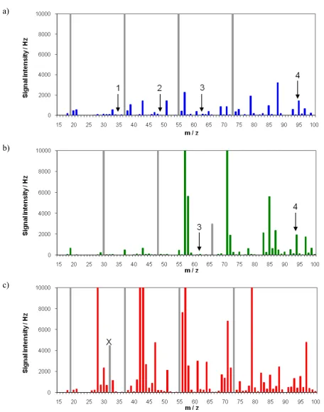
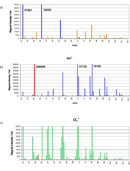
Figure 2.11 a) Analysis of Tedlar bags containing a known benzene concentration at different times. b) A large scale of the figure a showing the 10 ppb, the blank and the restricted concentration of benzene………. 46 Figure 3.1 SIFT-MS (Voice100) full scan data of the 1% natural gas in nitrogen
for the three ion reagents: (a) H3O+, (b) NO+ and (c) O2+ respectively. 1,2,3, and 4 corresponding to ion product mass peak position for hydrogen sulfide, methanethiol, ethanethiol plus dimethyl sulfide, and dimethyl disulfide. The grey lines indicate peaks arising from reagent ions and their cluster with H2O……….. 58 Figure 3.2 SIFT-MS (Voice100) full mass scan for liquefied petroleum gas (1%
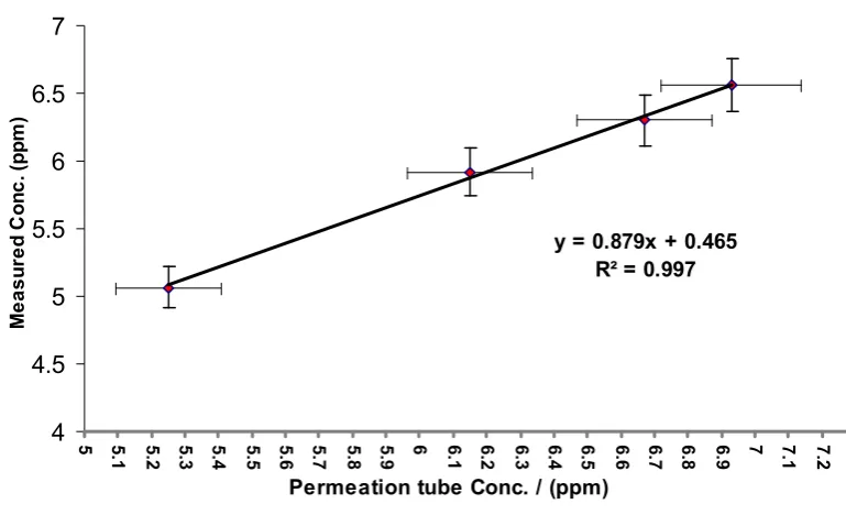
in nitrogen) for the three ion reagents: (a) H3O+, (b) NO+ and (c) O2+, respectively. The numbers 1,2,3, and 4 correspond to ion product mass peak positions for hydrogen sulfide, methanethiol, ethanethiol plus dimethyl sulfide and dimethyl disulfide. The grey lines indicate peaks arising from reagent ions with H2O. The “X” in (c) shows the severely depleted O2+ reagent ion signal……… 59 Figure 3.3 H2S calibration result, using the H2S permeation tube as a standard
concentration……… 61
Figure 3.4 Mass FullMassscan (Voice100) of undiluted natural gas for a) H3O+ b) NO+ and c) O2+, showing the high depletion of the reagent ions, and increasing number of the H3O+ cluster ions in part a. Figure 6.b is the chemical ionisation spectrum of NO+ and Figure 6.c has the same
spectrum for
O2+……… 63
Figure 3.5.a
The linear relationship result of H2S in a 1% mixture of LPG………… 65
Figure 3.5.b
The linear relationship exhibited for dilution of H2S in N2…... 65
Figure 3.5.c
The linear relationship exhibited for dilution of H2S in a 1% mixture of
natural gas……… 65
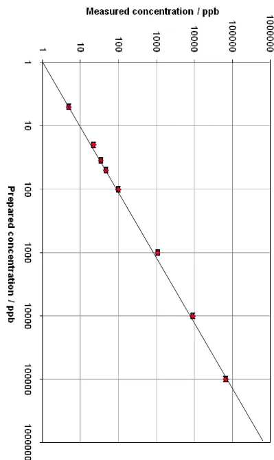
Figure 3.6 SIFT-MS quantitation of hydrogen sulfide in natural gas (1% in nitrogen) using the H3O+ reagent ion. Note that logarithmic scales are
used……….………. 66
Figure 3.7 Full mass scan of undiluted natural gas by (LDI1) using the low sample flow rate capillary for each of the three ion reagents (H3O+, NO+, and O2+). The mass scans derived from H3O+ and NO+ show good ion signals and are suitable for analysis. The mass scan, arising from O2+ , shows depleted reagent signal at m/z 32, indicated by red
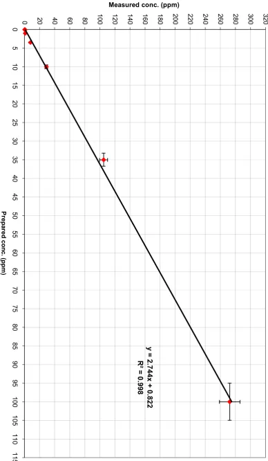
Figure 3.8 The different concentrations of H2S mixture with undiluted natural gas response on LDI1 using the low sample flow rate capillary. LDI 1 has not been calibrated for H2S, rationalising the different of the
concentration measured……… 70
Figure 3.9 Stability of the Standard 4.7 ppm concentration of the relevant
compounds over 3 days……… 75
Figure 3.10 The ICF function measurement 3days apart. b) Stability of the 35 ppb concentration of the relevant compounds over 4 hours in 1% LPG
mixture in N2……… 75
Figure 3.11 The linear relationship result exhibited for dilution of H2S, DMS, C2H5SH, and CH3SH in N2……….. 78 Figure 3.12 The linear relationship result exhibited for dilution of H2S, DMS,
C2H5SH, and CH3SH in 1% mixture of LPG………... 76 Figure 3.13 The linear relationship result exhibited for dilution of H2S, DMS,
C2H5SH, and CH3SH in 1% mixture of natural gas………. 76 Figure 4.1 The reaction of the 2-methylbutane with H3O+, NO+ and O2+(SIFT-MS
reagent ions)………. 81
Figure 4.2.a
The H3O+ full mass scan of 1% natural gas mixture in N2 using the Voice 200 instrument in which no halobenzenes were added (background). The blue lines represent the reagent ions………. 84 Figure
4.2.b
The NO+ full mass scan of 1% natural gas mixture in N2, using the Voice 200 instrument in which no halobenzenes were added (background). The red lines represent the reagent ions………... 84 Figure 4.3 The linear relationship between measured concentration and prepared
concentration for a mixture of bromobenzene and chlorobenzene in pure N2... 86 Figure 4.4 The linear relationship between measured concentration and prepared
concentration for a mixture of bromobenzene and chlorobenzene in a
1% LPG mixture in N2………. 86
Figure 4.5 The linear relationship between measured concentration and prepared concentration for a mixture of bromobenzene and chlorobenzene in a 1% natural gas mixture in N2 ……….. 87 Figure 4.6 The NO+ full mass scan for octane (C8H18). Different colors represent
Figure 4.7 The NO+ full mass scan for nonane (C9H20). Different colors represent
different concentrations...………. 92 Figure 4.8 Full mass scan for undecane (C11H24). Different colors represent
different concentrations...………. 92 Figure 4.9 The NO+ chemical ionization spectrum of sample 1. The GC-MS
spectrum of sample 1 is also shown………. 95 Figure 4.10 The NO+ chemical ionization spectrum of sample 2. The GC-MS
spectrum of sample 2 is also shown………. 97 Figure 4.11 The NO+ chemical ionization spectrum of sample 3. The GC-MS
spectrum of sample 3 is also shown………. 99 Figure 4.12 The NO+ chemical ionization spectrum and table of sample 4 product
ions identified. The 34 hydrocarbons in the sample are shown in the
table……….. 102
Figure 4.13 The NO+ chemical ionization spectrum and table of sample 5 product
ions identified………... 103
Figure 4.13.a
A summary of the 63 hydrocarbons present in sample 5 ………..…….. 104
Figure 4.14 The NO+ chemical ionization spectrum and table of sample 6 product
ions identified………... 105
Figure 4.14.a
A summary of the 89 hydrocarbons present in sample 1 …….….…….. 106
Figure 5.1 Monitoring results of the BTEX compounds in Christchurch as recorded in the 2005 ECan report. The dashed line in Figure A represents the current guideline value and the lower dashed line represent the 2010 guideline value………..………. 112 Figure 5.2 Seasonal analysis results of the BTEX compounds in Christchurch as
recorded in the 2005 ECan report……… 116 Figure 5.3 Passive sampling tubes, stainless steel and glass Tenax sorbent tubes… 123 Figure 5.4 a) Radial diffusive sampler design. b) Diffusive surface comparison
between axial and radial samplers c) Schematic illustration of the Perkin-Elmer axial passive sampling tube ……….. 124 Figure 5.5 Thermal desorber ATD 400………. 130 Figure 5.6 The residue of the compounds of interest in the tube before and after
the conditioning process……….. 135 Figure 5.7 TD-SIFT-MS desorption spectrum for a sampled spiked Tenax TA sorbent
Figure 5.8 SIFT-MS desorption spectrum for conditioned Tenax TA sorbent tube. 137 Figure 5.9 Recovery of relevant analytes and their average with experiment uncertainty
of ± 27%... 140 Figure 5.10 Air monitoring test at Syft Company’s backyard storage for period of 11, 25
and 33 days………. 141
Figure 5.11 Sketch diagram displays the passive sampling location next to the
SIFT-MS……….. 143
Figure 5.12 Workplace monitoring by real time SIFT-MS and passive tube with a) Tenax TA single bed sorbent b) Anasorb GCB1 and Anasorb CMS bed sorbents. c) Tenax and Carbopack bed sorbents………... 144 Figure 5.13 The three chosen sites: A) Coles Pl B) Woolston C) Riccarton ………. 145 Figure 5.14 Photos illustrate the sampling procedures that were taken……….. 146 Figure 5.15 A comparison of the analysis results of TD-GS-MS, TD-SIFT-MS and ECan
agency for JUL and AUG in 2008……….. 151
Figure 5.16 A comparison of the analysis results of TD-GS-MS, TD-SIFT-MS and ECan
List of Tables
Table Description
Page No. Table 2.1 Scotty bottle compounds that are used for the instrument calibration…..……... 27 Table 2.2 The relative decay rate of the three reagent ions with the maltol and the
collision rate of the H3O+……….. 34
Table 2.3 The resultant rate coefficients of the three reagent ions …...………...… 34 Table 2.4 Some of the milk flavour volatile compounds, including maltol, that are of
interest to the food and flavour industry……….. 35 Table 2.5 Citrus compounds of interest and their concentration in different citrus fruits… 40 Table 2.6 Concentrations in the background of different Tedlar bags, corresponding to
the designated analyte in ppbv ………. 43
Table 3.1 Important properties of sulfur compounds of interest according to NIST
chemistry webBook database……… 49
Table 3.2 Natural gas analysis components certificate, according to Southern Gas
Services Limited………... 51
Table 3.3 Hydrogen sulfide established dose-effect relationships……… 54 Table 3.4 H2S measured concentrations of the three systems by SIFT-MS comparing
with the prepared concentrations in Tedlar bag……… 61 Table 3.5 The LOD of the sulfur compounds of interest in natural gas (Voice 200)……... 77 Table 4.1 LOD values of bromobenzene and chlorobenzene in natural gas……….. 87 Table 4.2 Products of the reactions of NO+ with the given hydrocarbons. The Percentage
of each ion product is given in brackets…..……….. 93 Table 5.1 Guideline value of benzene and toluene compounds………. 110 Table 5.2 Physical characteristics of the compounds of interest……….. 120 Table 5.3 Tenax TA breakthrough volume for the compounds of interest………… 126 Table 5.4 Measured LODs for passive conditioned sorbent in a stainless steel tube:
(Conditioned tube-TD-SIFT-MS)………..……... 140
Table 5.5 The average weather conditions recorded during the sampling
Table 5.6 Literature uptake rate values and their average for the compounds of interest over a four-week period. ………...…….. 148 Table 5.7 Experimental measurements that confirmed the encountered dilution
Chapter 1
Introduction to SIFT-MS methodology
1. Introduction
In this chapter, by way of introduction, I will summarise the most important developments in the area of ion-molecule reactions with an emphasis on the experimental observations. This summary will be followed by some details of the Selected Ion Flow Tube Mass Spectrometer (SIFT-MS).
1.1 Ion-molecule reactions
Ion-molecule reactions have been noted, as early as the1913s. After the confirmation of the existence of gas phase ion-molecule reactions was reported by Dempster in 1916, many studies have been made in order to understand these charged gas phase neutral interactions. Ion-molecule reactions in the gas phase have been frequently found to proceed very quickly (on almost every collision) and with high efficiency. In addition, in the 1966s, Munson and Field realized the promise of these types of reactions as an alternative softer mean of ion generation. These two features, of rate and efficiency, have enabled ion-molecule reaction methodology to be applied to analytical applications.
Moreover, the rapid growth of the application was due, in part, to the precision of mass spectrometric identification of molecular weight information. Understanding these reactions has opened the door for them to be used in many applications. Further, the use of ion-molecule reactions provides a diverse frontier for extending the boundary of mass spectrometry. [1]
spectrometry techniques, all have important roles in understanding these reactions. Ion beam methods, for example, are being employed for the study of ion-molecule reaction dynamics including the elucidation of the energy dependencies of these reactions and the measurement of their reaction cross-section. [1] Flowing afterglow and selected ion flow tube are primarily used for measurement of rate constants of ion-molecule reactions and the identification of product ions. Ion-molecule equilibria enable the determination of thermo chemical information. Other kinetic aspects can be typically obtained from pulsed electron high-pressure mass spectrometers. Fourier Transform Ion Cyclotron Resonance Mass spectrometry (FTICR-MS) can also be used to study ion-molecule reactions with very high mass resolution mode, allowing the determination of molecular formulae of product ions.
1.2 Application of ion-molecule reactions
1.3 SIFT-MS
1.3.1 Overview
Selected ion flow tube mass spectrometry (SIFT-MS) can be considered as a sensitive analytical method. It is used for monitoring volatile compounds both organic and inorganic, based on the chemical ionisation principle to a very low concentration, parts per billion (ppb) by volume.
The technique evolved out of flow tubes used in physical chemical investigations of ion neutral kinetics before it was used in analytical chemistry. At Canterbury University, one of the areas of interest in the ion chemistry groups was understanding the astrochemical reactions that occur in the interstellar medium. The applications of flow tubes to ion molecule chemistry were begun by Ferguson and co-workers in 1969. [2] They applied the flowing afterglow technique to understand the ionospheric process occurring in the atmosphere. This technique then became a standard method for the study of the ion-molecules reaction at thermal energies. [3]
The flowing afterglow method is a fast flow tube ion swarm method for the study of the reactions of positive and negative ions with atoms and molecules. It has been extensively used to study ion molecular reaction kinetics and has had numerous applications to atmospheric and interstellar ion chemistry over a 20 year period. In this period many polyatomic and diatomic cations have been found to exist in the interstellar medium by the use of radio astronomy methods.
flowing afterglow technique, when applied to ion-neutral chemistry, was the combination of all positive ions, negative ions and electrons together in the flow tube, making identification of the production difficult. This problem was addressed by Smith and Adams [6] who introduced a second quadrupole mass spectrometer to select the ion whose reactions were to be studied. This modification became known as Selected Ion Flow Tube, SIFT.
Recently, the SIFT technique underwent a further development as a sensitive analytical technique for the quantification of the trace gases in air and human breath, down to the pptv level in real time, using chemical ionisation. [7] This new development in analytical chemistry is known as SIFT-MS. The initial larger SIFT instrument, in the Department of Chemistry of the University Canterbury, was modified for use as a SIFT-MS instrument in the late 1990s. Then, a purpose built smaller SIFT-MS instrument was constructed. This became the property of Syft Technologies Ltd on its formation in 2002. Early in 2004, Syft Technologies Ltd commissioned a new SIFT-MS specifically designed for the analyses of trace volatile organic compounds (VOCs). Subsequently, the Voice 100, first generation of SIFT-MS, was released to the commercial market in November 2004 followed by Voice 200 in late 2007.
1.3.2 SIFT-MS Instrument
1.3.2.1 Ion source region
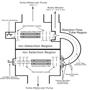
[image:21.595.115.419.73.427.2]The ion source region is where the ions are created before they are transmitted to the reaction region. This region can be divided further into two sub-regions, the ion creation region and the ion selection region. In the ion creation region, ions are generated under 0.3 Torr pressure by using microwave discharge, operating on moist air. The air is made moist by adding water from the water reservoir that is held inside the machine. The ions generated from this source are H3O+, NO+, and O2+ and are the most thermodynamically stable ions. Figure 1.2 shows the mechanism for generating these ions and their energy. Once formed, these ions are focused by electrostatic lenses into the quadrupole mass filter in the ion selection section. The quadrupole mass filter enables the selection of specific ion precursors for more analytical
advantages. That is, SIFT-MS allows each ion of interest to be selectively injected into the reaction region with a rapid switching time < 10 ms between the three ions. After the mass selection, the reagent ions are injected into the ion reaction region.
1.3.2.2 Ion reaction region
wide and is 4.35 mm outside the ion aperture. The outer annulus is 0.4 mm wide at a radial distance of 37.1 mm from the ion aperture and is used to introduce the second carrier gas, argon. Helium is passed through the inner annulus at 15 Torr L s-1, creating the Venturi effect that helps to inject the ions into the flow tube against the pressure gradient. The argon, on the other hand, is passed through the outer annulus slit at 25 Torr L s-1.
Furthermore, the flow tube has five inlets connected to it for transmission of various gases and vapour mixtures. The tetradecane inlet, ambient air inlet, calibrant inlet, direct inlet and sample inlet are connected to the flow tube for different tasks. For example, a quadrupole mass calibration can be done by using the tetradecane inlet, which adjusts the mass peaks to the known tetradecane mass peaks.
Many parameters have to be taken into account in order to determine the analyte concentration. The carrier gas flow rate, ion velocity, sample flow rate, relative diffusions of the reagent ions and product ions and the flow dynamics of the gas inside the flow tube, all have to be known for reliable analytical measurement to be achieved.
1.3.2.3 Ion detection region
1.3.2.4 Quadrupole mass filter
Quadrupole mass analyzers are currently used most frequently by chemists to obtain the molecular weight, particularly in chemical analysis. This device has significant advantages over other traditional mass analyzers, although it is not a high-resolution device. It is a relatively low cast device and couples readily with the detectors. It is also widely used with GC-MS and LC-MS instruments.
Resolving ions by this technique is based on the ion mass to charge ratio (m/z) rather than momentum or kinetic energy. [8] Another useful feature in the quadrupole mass device is the mechanical simplicity of the instrument. It does not rely on the use of a magnetic field in mass discrimination, avoiding the conventional magnetic field problems, such as the weight of the instrument, the cost and slow scan speeds. Moreover, the resolution of the quadrupole is set electronically rather than mechanically. Therefore, and in light of the previous advantages, it seems to be an ideal instrument for remote and fast analytical applications.
Physically, the quadrupole consists of four electrodes that are accurately positioned in a radial array making a circular cross section, as shown in Figure 1.3.
DC and RF potentials are applied in these electrodes in order to control the ions' passage to the detector. Therefore, when the RF is positive in regard to the centre axis, a beam of positive ions will be accelerated and focused onto the center axis of the electrodes’ structure. On the other hand, when negative RF is applied, the ions will be accelerated toward the negatively biased electrodes. The combination of both RF and DC potential will affect the trajectory of the collection of ions on the quadrupole. So, by controlling the RF and DC potential, a mass spectrum can be achieved. By appropriate controlling of the RF/DC ratio, ions will be filtered based on their mass to charge ratio. Consequently, mass resolution of the device is governed by the ratio of the RF to DC potential, applied to the electrodes.
Another effect that needs to be accounted for is related to ion mass. The heavier ions' count rate is enhanced by lower differential diffusion away from the flow tube axis and diminished through the discrimination effect in the quadrupole. In contrast, the light ions' count rate is diminished through diffusion away from the flow tube axis and enhanced through the quadrupole discrimination. These two phenomena therefore tend to cancel each other out, but they must be appraised for accurate analysis.
The DC-RF stability diagram provides a powerful method of visualizing the operation of the quadrupole mass filter at the different voltages. Moreover, it is used to set the scan line when the instrument mass scale is calibrated.
1.3.2.5 Einzel lenses
These electronic lens arrays are used for refocusing the ions before entering the quadrupole mass filter, in both the upstream and downstream chambers. An array of these lenses is set before and after the quadrupole, with an overall negative voltage gradient for adjusting and alignment purposes. This is in order to optimise the number of ions reaching the detector and hence to maximise the ion signals. These lenses are illustrated by Figure 1.4.
A high negative voltage is used in the first two lenses of the ion source region with the aim of: breaking the plasma sheath; pulling the positively charged ions out of the static plasma and also reducing the ion-electron recombination in the plasma, which is very fast.
1.3.2.6 Multiplier
An electron multiplier is used in the end of the downstream chamber, for detecting the ion signals. It converts single ions into a measurable electrical pulse. This type of electron multiplier has been used widely to detect charged particles either positive or negative, especially in analytical instruments, for more than 30 years. [9]
The multiplier is a vacuum tube-type structure that multiplies incident charges. This tube is often built as a funnel of glass coated inside with a thin film of a semi-conducting material.
For positive ion detection, a negative high voltage is applied at the wider input end. A small positive voltage near the ground potential is applied at the narrower output end, as shown in Figure 1.5. When the ion is bombarded on the funnel, electron emission is induced. Then, the large potential gradient on the surface accelerates the electron with the process being repeated many times over, creating an avalanche of secondary electrons. A typical gain of an electron multiplier is 5×10⁷. The ion signal on the output is then counted by a pulse amplifier discriminator unit. [10] The particle multiplier used in the SIFT-MS Voice100 is a DeTech model 203. [11] One drawback, when very high ion count rates are experienced, is that successive pulse may not be able to be resolved. This however, is unlikely to occur at the count levels that are typical of a Voice 100 instrument.
1.3.2.7 Pumps
Specific conditions have to be maintained in the SIFT-MS instrument to make it operate and transmit ions. Pressure is one of the critical conditions for the operation of the mass spectrometer. The high voltages required for the detector, lead to internal discharges at low to moderate pressures. They must be operated below 10-4 Torr. Thus, different types of pumps are coupled to the instrument for getting the right pressure conditions that are needed. Each region in the instrument needs a particular pressure. The upstream and downstream chambers
require very low pressure in order to allow molecules to flow. For this reason, a high capacity pump is required to achieve the very low-pressure needed for maintaining a flow pressure and reducing the number of collisions. For both chambers, a turbo molecular pump has been chosen for this task. The turbo molecular pump has the capacity to go to very low pressures of 10-5-10-8 Torr and at speeds of 150-2500 L/s. This pump has a series of vaned blades on a shaft, rotating at speeds up to 60,000 rmp between an alternate series of slotted stator places (Figure 1.6). Air, as described in McMaster's book [12], is grabbed by the blades, whipped through the stator slots and grabbed by the next blade. In this process, although only a small amount of air is moved each time, the number of blades and high rotary speed rapidly move more air from the chamber to the exhaust. In addition, the biggest advantage of using the turbo pump rather than the oil diffusion pump, which operates in a similar process regime, is that it contains no oil to contaminate the analyzer.
However, some conditions are required to make the turbo pump operate at the high rpm rates required. These high rotational speeds can only be achieved by providing the turbo pump, backed by another pump, with less capacity to lower the pressure at which it operates. This backing pump is a rotary vane vacuum pump (Figure 1.7) and has the capacity to take the pressure down to 10-3 Torr, which is required for the turbo to operate. This pump has the capacity of moving 50-150 L/min. A further pump is required to achieve the flow speeds necessary for the flow tube gas at 0.5 Torr. A Roots pump, backed by a rotary vane pump, is used for this purpose.
[image:29.595.302.497.86.339.2]
[image:29.595.64.180.139.317.2]
Figure 1.8 A detailed schematic diagram of the Voice 100 SIFT-MS.
[image:29.595.146.450.407.719.2]1.3.3 How SIFT-MS works
After turning the instrument on and getting to the right operating conditions, ion precursors are generated to give the most stable positive ions: H3O+, NO+ and O2+. These ions are focused by the lenses, into the quadrupole mass filter. At that stage, a specific ion of interest is selected by the quadrupole mass filter. The ion of interest is refocused again by the next lens array and injected into the flow tube in which the pressure is higher than the upstream source chamber pressure. These ions are passed to the flow tube taking advantage of the Venturi effect from the venture nozzle. After that, these ions undergo many collisions with the bath gas in the first few cm of the flow tube. In this thermalising process, the excess energy is removed from the excited ions, transferring most of them to the ground electronic state and thermal velocity distributions as illustrated in Figure 1.9. The presence of the excited ions can lead to different ion products and can affect the reproducibility of the system. Excited NO+ has only been found in small quantities of about 2% in the flow tube. However, the thermalization process still seems to be very effective. Then, the ions are carried by both carrier gases, argon and helium, inside the tube, colliding with neutral compounds that are inserted from a heated capillary in the sample inlet. Argon is used in this instrument for its advantage of reducing the radial diffusion of ions in the tube. [13]
Figure 1.9 Sketch illustrates the thermalizing ions region
Detection
Region
Thermalizing ion region
1.3.4 Important Points that must be considered when using SIFT-MS
There are some important points that have to be considered when dealing with SIFT-MS in order to have accurate and precise measurements. Firstly, the applicable concentration range of the SIFT-MS for the quantization analysis of molecules has to result in a less than 15% reduction in the precursor ion signal as a consequence of the reaction with the analyte. Secondly, the uneven loss of ions according to mass through the instrument can lead to inaccurate measurements and has to be corrected. The diffusion phenomenon and mass discrimination variation of the quadrupole, perhaps, are the most contributing phenomena to the loss of the unit efficiency of this system. However, the radial diffusion losses, away from the flow tube axis, are reduced by using argon gas. [13] Therefore, a correction is essential for achieving good results considering these phenomena. Based on that, an instrument Figure 1.10 SIFT-MS outcome spectrum, indicating the main and secondary ion precursor peaks
H3O +
NO+
O2 +
H3O +
.H2O
H3O +
.(H2O)2
H3O +
calibration is usually done to correct the ion signals. Two different methods have been used to measure the instrument calibration factor (ICF), which will be discussed later. However, the SIFT-MS technique does not require a calibration to be carried out on a per-analyte basis.
Thirdly, downstream quadrupole stability has to be checked in order to hold the signal in a fixed position as a function of time and increasing temperature of the instrument. This can be checked by selecting a specific mass signal, monitoring the movement of the signal for a period of time and by increasing the instrument temperature, using 10 steps per a.m.u. scan.
Fourthly, the capillary and sample flow rate are also very important in terms of their effects on the analytical measurements. The sample flow rate has to be preset to reach the desired good results. In addition, there is another problem in introducing the sample to the capillary, which is the adsorption of the analyte compounds on the capillary walls. Heating the capillary has been found to reduce this phenomenon; it minimizes the loss of condensable trace gases by surface adsorption but does not completely dominate the problem for “sticky” molecules. A better solution is to use a passivated capillary and inlet system in order to reduce the adsorption and to produce a linear relationship between the concentration and the count rate.
1.3.5 Ion molecule reactions
The three most common ion-molecule reactions that have been noted with the SIFT-MS ion precursors, H3O+, NO+, and O2+, are proton transfer, charge transfer and dissociative charge transfer, and ion precursor association reactions. H3O+, NO+, and O2+ are considered the best ions of choice in most analysis cases because of their prominence in an air afterglow in the SIFT-MS ion source. These ion reagents are not highly reactive with the major components of air. Their use can allow some mass identification of VOCs, unlike the PTR-MS, which mainly uses H3O+. Further, a combination of these ion precursors facilitates the determination of many of the compounds of interest. At the same time, they resolve many of the interference problems and add some extra complementary information.
1.3.5.1 H3O+ reactions
H3O+ can be deemed the most common ion precursor for quantifying polar organic compounds. Generally, most reactions proceed mostly via exothermic proton transfer as exemplified in reaction 1. An important feature of this reaction is that it mostly proceeds with unit efficiency.
H3O+ + M MH+ + H2O (1)
formed, in parallel, in some cases, so a careful search must be made to determine all the product ions. More complex product ions formation has been found with ether and ester reactions.
In addition, the formation of water clusters, as indicated by equation 2, can provide secondary reactions that need to be included in the analyte quantification process and also increase the complexity of analyzing the spectrum peaks. The wetter the sample, the greater the role of secondary reaction of the product ions with H2O. A dihydrate is usually formed with alcohols, aldehydes and carboxylic acids, while a monohydrate is usually formed with ketones, esters and ethers, as indicate in equation 3.
H3O+ + H2O + X H3O+.(H2O)n + X (2) X is third body (He or Ar)
H3O+.(H2O)n + M MH+.(H2O)n + H2O (3) ligand switching reaction
MH+ + H2O MH+.(H2O)n
The molecular species that have a lower PA than water cannot undergo proton transfer reaction and for these analytes other ion precursors are required.
1.3.5.2 NO+ reactions
The reaction with NO+ undergoes three types of reactions: association, charge transfer, and hydride ion transfer. The charge transfer reaction occurs when the ionization energy (IE) of the compounds is smaller than the ionization energy of NO+, 9.26eV. It occurs with aromatic hydrocarbon and organosulfur molecules [14][15] as equation 4 illustrates.
Association reactions, in contrast, commonly occur with some types of polar organic molecules especially carboxylic acids, esters, and ketones. They often occur in parallel with other processes. This reaction is apparently enhanced when there is not much difference between the IE of the NO+ and the IE of a compound such as some ketone, where the IE of the acetone, for example, is 9.71eV as shown in equation 5 below.
NO+ + CH3COCH3 + He NO+CH3COCH3 + He (5)
Finally, the hydride ion transfer reaction is the only process that occurs specifically with NO+. This involves the abstraction of H- from the compound, resulting in HNO and a single ion product, the parent cation molecule with less H (see equation 6), particularly with aldehydes, ethers, and primary and secondary alcohols.
NO+ + CH3CHO CH2CHO+ + HNO (6)
1.3.5.3 O2+ reactions
Most of the O2+ reactions are direct charge-transfer reactions (equation 7) and dissociative charge-transfer reactions (equation 8). The O2 molecule has an IE of 12.06eV. Accordingly, the O2+ will react with most molecules having lower IE. As the IE of O2 is appreciably greater than most organic compounds, it reacts with many molecules via one of the above processes.
O2+ + M M+ + O2 (7)
O2+ + C4H10 C4H10+ + O2 (8)
C4H9++ O2 + H
C3H7++ O2 + CH3
Using O2+ ions in the SIFT-MS reactions leads to multiple ion products and therefore a more complex mass spectrum. It is similar to the mass spectrum obtained by electron impact ionization that results in extensive fragmentation of the parent molecule. The number of products generated by O2+ chemical ionization limits the usefulness of this precursor. O2+ is most valuable for the detection of inorganic volatile compounds such as NO, NO2, NH3 and CS2 in which it does not undergo dissociative charge transfer with these species. Moreover, it is also useful for checking the identification of the H3O+ and NO+ products.
1.3.6 Kinetics and rate coefficients
A fundamental requirement of the SIFT-MS technique is the knowledge of the kinetic parameters of the reagent ions with the analyte molecules. Consequently, the rate coefficient and the product branching ratios need to be determined for the reagent ions’ reactions with all the compounds of interest.
Two methods have been used to measure the rate coefficient. [11] Firstly, the absolute method, in which the rate coefficient is obtained from the slope of the semi-logarithmic plot of ion intensity against an absolute measurement of neutral flow for compounds with vapor pressure greater than ~2.5 Torr at 20 °C.
The rate coefficient from this method can be determined theoretically from the simple chemical reaction equation:
A+ + B products
The rate reaction between A+ and B is given by
Because [B] >> [A+] by typically 5 orders of magnitude. This rate law can be defined as a pseudo-first order rate law.
By integrating this equation, we have:
[A+] =[A0+]exp(k[B]t)
ln[A+] =ln[A0+]-k[B]t
[B] is the number density of the ion precursor. [B] can be determined from the flow rate as the next equation shows: [7]
[B]=
[B] = number density, Kb = Boltzmann constant, Tg = carrier gas temperature, ΦR= reactant gas flow rate, Φc= carrier gas flow rate, Pg=carrier gas pressure.
So, the integrated equation can be expressed in terms of the intensity, as shown below. lnI=lnI0-kt[B]
Then, this equation can be written in terms of the correction, as shown next.
lnI=lnI0-k[B]
I= count rate of the precursor, I0= count rate of the precursor in the absence of the analyte, k= rate coefficient, [B]= number density, ε= end correction distance, mixing distance of the reactant gas into o the carrier gas that is typically 2cm, γi= ion velocity, l = the distance of the inlet port to the downstream orifice.
The second method is a relative method, which is used for compounds with vapor pressure less than 2.5 Torr at 20 °C. In this method, only the rate coefficient is measured relative to the H3O+ reaction, which is assumed to occur at the collision rate. This method depends on the knowledge that exothermic proton transfer reactions proceed at the collision rate and there is extensive laboratory evidence to support this view. The collision rate can be calculated theoretically if the polarizability and the dipole moment of the reactant molecule are known.[16] Then, from the ratio of the decay rates of the NO+ and O2+ reactions compared to the decay of H3O+, rate coefficients can be determined for NO+ and O2+.
In summary, if the rate coefficient and product ion ratios are known, then the concentration of the analyte can be determined. Thus, knowledge of the product ions and their kinetic data is loaded into the software database used by the SITF-MS instrument, which then can be used for an analyte concentration measurement.
1.3.7 Modes of operation of SIFT-MS
Two instrument modes can be used in the SIFT-MS experiment: the mass scan mode and selected ion monitoring scan mode (SIM). As mentioned in the GC-MS A Practical User’s
Guide Book, the difference in these two modes can be described as: “it depends on whether
we wish to look at the forest or the trees.”
1.3.7.1 Mass scan mode
1.3.7.2 SIM scan mode
In SIM scan or selected ion-monitoring scan, only pre-selected masses are scanned rather than scanning the full mass range. In other words, it is a jump scan over a discrete number of masses. [18] This mode gives more accuracy in terms of the ability to monitor specific ion amplitude. It can be used for all three-reagent ions during a single SIM scan.
Chapter 2
Preliminary preparations and experiments 1. Introduction
Before performing experiments, a thorough series of calibration checks of the instrument are required. This chapter describes the experimental procedure followed during the course of preparing the instrument prior to use for analysis. This procedure is important in terms of obtaining reliable measurements. Then, this discussion is followed by a brief summary of experiments on some important flavour compounds, and an examination of the validity of using Tedlar bags for air analysis. These introductory experiments provide more insight into instrument-required procedures, and appraise the ability of this technique to cope with potential problems associated with a range of analytes.
2. Preliminary work
This research began from preliminary tests in the laboratory with the SIFT-MS to test the validity of the current parameters of the instrument. This, in fact, included calibrating the instrument, measuring the instrument calibration factors (ICF) and testing the quadrupole stability of the instrument. Then, the compounds of interest were calibrated for better measurement accuracy.
2.1 Instrument calibration
2.1.1 Instrument calibration factors ( ICF)
i. The Constant Cumulative Count ( 3C method)
The 3C method is based on the assumption of normalising the sum of all detected ion signals over the entire mass range, if there was unit transmission and detection efficiency for all ions passing through the instrument, regardless of the product-ion distribution. The 3C method simply involves producing a number of mass spectra with different product-ion distributions and then choosing a function of mass that, when applied to those mass spectra, show a constant sum of all product signals that match the unreacted reagent ion's signals. The outcome of this procedure is that if the ICF is correctly applied, the same ICF will also be true in the presence of mass discrimination effects. The 3C method was performed according to the Syft procedure by making samples of a selection of analytes that result predominantly in a single product ion, at the chosen concentration in the mass range of the instrument. Also, the concentration of these analytes should be concentrated enough to reduce the reagent ion count by more than 20%, but not so concentrated that they influence the diffusion of ions in the flow tube. The following samples were used as they had been shown to give satisfactory results:
a. Sample inlet closed g. Xylene
b. Nitrogen with a trace of moisture h. Acetone c. Air at the ambient humidity i. MEK d. Air at breath humidity j. Pentanone
e. Benzene k. Hexanone or MIBK
f. Toluene l. Heptanone
New calibrated cylinder method for determining ICF
The new ICF method is based on using predefined analyte concentrations such as, measuring concentrations present in a Scotty bottle that contains compounds known to a high precision. These compounds have different mass ranges, with the range of compounds used covering the entire mass spectrum required as shown in Table 2.1.
Table 2.1 Scotty bottle compounds that are used for the instrument calibration.
Analyte M.Wt
C2H4 28
C4H10 58
C6H6 78
C8H10 106
C4H2F4 126
C6F6 186
C7F8 236
The signal intensity can be adjusted according to the mass of the analytes used. Theoretically, this can be explained by the following: first, the concentration of a known analyte is measured; the concentration, as determined by the SIFT-MS instrument, is then adjusted to the correct concentration according to the equation below:
kt I
P A
ICF ICF
+ +
=
]
[
Where:
[A] is known and k, I+ and P+ are known parameters. One parameter, t, the time of the reaction in the flow tube, still has to be determined before the ICF can be measured. The reaction time t, can in fact, be measured from the ethene reaction (equation 1) with O2+ where ICF is assumed to be 1 for both the O2+ and C2H4+ ions that have masses of 32 and 28 respectively. This is due to the small mass discrimination between O2+ and C2H4+, which assumes ICFO2+≈ ICFC2H4+=1. Therefore, in this case the only unknown parameter is t, which then can be easily calculated. The reaction time is assumed constant for all reactions, so the only parameter left unknown is the ICF. The ICF product factors are measured for the compounds that are illustrated in Table 1 above, and range up to 186 amu for the Voice 100 instrument.
C2H4+ O2+ C2H4+ + O2 (1)
0 1 2 3 4 5 6 7 8
0 50 100 150 200
Mass
C
o
r
r
e
c
t
io
n
ICF During Calibration Desired ICF Setting
+
O2++
+
O2
C6H6 + H3O+ C6H6.H+ + H2O (3)
Figure 2.1 ICF diagram result for the LDI1 instrument, using the new cylinder method.
2.1.2 Quadrupole stability
The stability of the quadrupole mass filter is very important in quantitative analysis. This stability was tested on the voice 100 (P1) instrument in order to establish the reliability of the data, by monitoring a specific mass as a function of temperature and time. It is expected that the position in mass spectrum should be constant to within ±0.1 amu. To do this, the mass scan line was first calibrated using tetradecane (C14H30). The instrument was then switched
Mass ICF
19 1.2
28 1
31 1
57 0.84
78 1.03
106 2.03
150 5.7
186 7.5
3000
2500
2000
1500
1000
500
0
128.0 127.5
127.0 126.5
126.0
Mass / amu
126.75
126.70
126.65
126.60
126.55
M
a
s
s
/
a
m
u
2.0 1.5
1.0 0.5
0.0
Time / hr
33
32
31
30
29
T
e
m
p
/ d
e
g
C
drift
Tube_Temperature__C_
off to allow it to cool down for about 2 hours. It was then turned on again and the quadrupole stability was tested using a repeating scanning method, as a function of time and temperature. Movement in mass peak of more than 0.1 amu, as shown in Figures 2.2 and 2.3, is an example of an unstable quadrupole mass filter as found in the P1 instrument, prior to the adjustment of the RF transforming voltage of the planar with increasing temperature. Figures 2.4 and 2.5 show a good stability of the quadrupole with reproducibility in the mass position better than 0.1 amu.
Figure 2.2 Unstable quadrupole, band signal shifts more than 0.1 amu
2500
2000
1500
1000
500
0
127.0 126.8
126.6 126.4
126.2 126.0
Mass / amu
126.58
126.56
126.54
126.52
126.50
M
a
s
s
/
a
m
u
1.0 0.8
0.6 0.4
0.2 0.0
Time / hr
25.5
25.0
24.5
24.0
23.5
23.0
T
e
m
p
/
d
e
g
C
drift
Tube_Temperature__C_
Figure 2.4 Reproducibility of a mass peak in stable quadrupole, showing shifts in the mass of less than 0.1 amu.
2.2 Analyte calibration
Recently, with the ongoing developments in analytical methods for sampling, a number of different methods is available for preparation of calibration mixtures. Two methods have been used in this work for preparing standards. [20]
2.2.1 Static method
In the static method, the sample is prepared by injecting into a container, a known weight of the target organic compound that is sufficiently volatile to be completely vaporized. This method, nonetheless, shows certain drawbacks in terms of the degree of the stability of the compound in the container; the adsorption process by the container wall and errors introduced in the dilution steps.
2.2.2 Dynamic method (Permeation tube)
In contrast, dynamic methods are generally preferred for generating standard mixtures using permeation tubes. Several advantages have been noted for this method according to Simonetta et al.’s study (2005) [21], such as minimizing the effect of adsorption, the capability of producing precise continuous dilution ranges and the ease of generating flow having different humidity.
Permeation tubes contain gases that have usually condensed to liquids under pressure. The weight loss of vapour through the walls of the tube, at the specified temperature, has been evaluated by the manufacturers. When operated at the temperature specified, they can be used as primary calibration standards.
3. Some important flavour compounds analysis
3.1 Maltol
Maltol is a natural organic compound that is used primarily as a flavour enhancer. It is one of the flavour compounds in milk and cheese and is one of a range of other important flavour volatile compounds that the food and flavour industry are interested in, as shown in Table 2.4. In order to measure its concentration in milk and cheese, using the SIFT-MS technique, we have first to determine the kinetic parameters of the main reagent ions H3O+, NO+ and O2+ with maltol. In order to obtain these parameters for maltol, the relative rate method is used because of the low vapour pressure of maltol (2.43×10⁻⁴ Torr at 25 °C). In this method, a diluted sample of maltol was created in a Tedlar bag full of nitrogen and then sampled into the SIFT-MS. Next, the products arising from the reaction of each reagent ion with maltol, were identified and counted. Relative decay rates were then obtained for each reagent ion. For example, the reaction with the H3O+ produces one proton transfer ion product. Further, it
3-hydroxy-2-methyl-4H-pyran-4-one
M.Wt. 126 g/mol
is known that the rate of this exothermic proton transfer reaction equals the collision rate, as this invariably occurs for exothermic proton transfer reactions.[22] This rate can be calculated theoretically with regard to the dipole moment and the polarizability of the maltol.[16] The rate coefficients for the reagent ions NO+ and O2+, cannot be obtained by the same calculation because their reactions do not necessarily occur on every collision. However, their rate coefficients can be obtained by measuring their decay rates, relative to that for H3O+. The result is summarised in Tables 2.2 and 2.3.
Table 2.2 The relative decay rate of the three reagent ions with the maltol and the collision rate of the H3O+
H3O+ NO+ O2+
k 5.41 2.42 2.91
% 100% 45% 54%
H3O+ Collision Rate
4.8×10-09
Table 2.3 The resultant rate coefficients of the three reagent ions.
Precursor Rate constant
Compound Sensory properties[23]
Chemical structure M.Wt
Skatole Flowery 131.17
Acetone 58.08
2-heptanone Blue cheese 114.19
Maltol Caramel 126.11
2-Hepten-1-al Oily , putty 112.17
2-Heptenal,Z Oily , putty 112.17
2-Heptenal,E Oily , putty 112.17
Ethyl butanoate Ester, fruity 116.16
2-Methyl butanal Malty , cocoa 86.13
Table 2.4Some of the milk flavour volatile compounds, including maltol, that are of interest to
3-Methyl butanal Malty, cocoa 86.13
Dimethyl sulfide Cowy 62.14
1-Octen-3-one (Vinyl amyl
ketone)
Metallic,
mushroom 126.20
3.2Distinguishing between aldhydes and ketones
SIFT-MS has the ability to distinguish between some isobaric compounds. This is a valuable asset when applied to aldhydes and ketones, which are very common components in food flavours. To do this, the selected ion precursor feature is used. Butanal and butanone, which have the same molecular mass of 72 amu, are distinguished by using a particular precursor and looking for different product masses as a consequence of different reactions of aldehydes and ketones with the reagent ions. The reaction with H3O+ gives the same product ion mass for both of them at mass 73 and therefore cannot be used for distinguishing between them. However, the reaction with NO+ gives an association reaction with butanone to give a 102 amu product ion and hydrogen elimination with butanal, giving a product ion at 71 amu. Therefore, the reaction with NO+ provides a convenient way of distinguishing between these isomers as shown in the following equations:
C H3
CH3 O
+ NO+ C4H8O.NO+ (102 amu)
H C
H3
O
+ NO+ C4H7O+ (71 amu)
Butanone
This distinction between butanone and butanal was utilised when examining a sample of a liquid coffee, which had a complex aroma. Coffee is known to contain over 500 compounds that have been observed in the headspace using different analytical techniques. Two of these compounds are butanone and butanal. A diluted butanone solution was added to a liquid coffee sample and the relationship between an added quantity of butanone in the coffee and in the headspace was measured using the SIM method with NO+ as the reagent ion. A linear relationship was obtained as shown in Figure 2.6. This linear result confirms the fact that butanone can be distinguished from butanal in a headspace of a liquid coffee mixture and shows the linear response.
The experiment conducted on coffee demonstrates how SIFT-MS is able to distinguish between isobaric compounds with different functional groups such as ketone and aldehyde.
3.3Vanillin
Some work was done on vanillin, which is one of the compounds that can be found in several different foods. Vanillin is also commonly added as a flavour compound in foods, so having the ability to detect it is very important to the food industry. However, an immediate problem arose when dealing with this compound with its 3 different functional groups. This problem was mainly related to the inability to measure the exact concentration of the compound because of its adsorptive nature on the walls of the inlet. Hence, the sticky property of this compound led to a reduction in the ion count of the product. The degree of adsorption was investigated. A set of different vanillin concentrations, in a range of ppm concentrations, was prepared for quantitative analysis in an attempt to achieve a linear relationship between increasing concentration and the headspace ion count. A short heated inlet was used in this process to avoid the exposure of vanillin to a large surface area, as this tends to reduce the sticky effect of the vanillin. The result, nonetheless, was not satisfactory as illustrated in Figure 2.7. It indicated a significant extent of vanillin adsorption on the inlet walls that increased in proportion to the concentration of vanillin. Significant deviations from headspace concentration and solution concentration were apparent.
Benzaldehyde, 4-hydroxy-3-methoxy
Figure 2.7 Vanillin deviating concentration due to adsorption process.
4 Citrus fruits experiment
Some experiments were performed on citrus fruits in order to determine the concentration of specific compounds, in different types of citrus. These compounds make up the distinctive aroma of citrus fruits and many of them are common to a number of citrus fruits. The ratios of the different citrus fruit compounds determine the unique bouquet of the different fruits. The method that was used in these experiments was the selected ion method (SIM). This method scans selected masses of relevance to target compounds. It is suitable for accurately determining the concentration of each targeted analyte. The experiment was done using the same quantities of lemon, orange, grapefruit and mandarin. Roughly, 20 grams of each were placed into 1.5 litre bottles and sealed with a septum. The results are shown in Table 2.5 and graphically in Figure 2.8.
0 10 20 30 40 50 60 70 80 90 100 ger an ial ge ran iol lin alo ol ac eta lde hyd e eth yl ac eta te eth yl p
rop ion
ate
eth yl b
uty rate citr on ella l eth yl 2
-m eth ylb uty rate eth an ol lim on en e oct an al thym ol me thy l N -m eth ylan tha nil ate hex an al tra ns -2-h exe na l hex en ol iso pe nty l alc
oh ol gra pef ruit m erc ap tan C o n c e n tr a ti o n / p p m labair background grapefruit lemon orange mandarin Concentration (ppm) Compounds
lab air background grapefruit lemon orange mandarin
Geranial 0.005 0.005 0.15 0.005 0.058 0.014
Geraniol 0.002 0 0.092 0.019 0.061 0.014
Linalool 0 0.002 0.3 0.15 0.33 0.12
Acetaldehyde 0.013 0.01 7.6 2.2 6.9 4.8
Ethyl acetate 0.006 0.006 9.4 0.081 0.13 0.27
Ethyl propionate 0.006 0.003 0.17 0.11 0.099 0.12
Ethyl butyrate 0.038 0.026 0.71 0.22 0.17 0.074
Citronellal 0.002 0 0.13 0.005 0.041 0.013
Ethyl 2-methylbutyrate 0 0 0.054 0.014 0 0.004
Ethanol 0.25 0.24 96 11 63 27
Limonene 0.009 0.013 80 29 80 39
Octanal 0.001 0.002 0.021 0.001 0.011 0.008
Thymol 0.001 0.005 0.045 0.022 0.019 0.01
Methyl N-methylanthanilate 0 0 0.048 0 0.017 0
Hexanal 0.006 0.005 1.3 0.12 0.71 0.29
Trans-2-hexenal 0 0.001 0.19 0.043 0.12 0.08
Hexenol 0 0.002 0.016 0.004 0.007 0.009
Isopentyl alcohol 0.003 0.004 0.009 0.002 0.007 0.006
Grapefruit mercaptan 0.007 0.004 0.028 0.004 0.013 0.009
5. Tedlar bags
Several methods are used to store samples and transport them to the laboratory such as canisters, cold trapping, Teflon bags and Tedlar bags. Tedlar bags are particularly convenient for holding samples because of their ease to operate, to handle, their low cost, and their re-usability. However, some problems were found when dealing with these bags. Concentration stability of contents in these bags for a number of compounds is not very satisfactory. Some analytes appear to increase their concentration with time but more commonly, others show a decreasing concentration with time. Tedlar bags also have significant concentration of several compounds arising from the bag polymer. For example, some compounds present in the bags are produced by the bag material itself including, N-N-dimethylacetamide (C4H9NO solvent used in the production of the Tedlar bags) and phenol at m/z 88 and 95 amu respectively. These compounds also increase with increasing temperature. In their study of monitoring the effect of temperature on Tedlar bags, Marco et al. found an increase in the concentrations of these species 170% (C4H9NO) and 88% (phenol).[25] Therefore, this contamination affects the analyses results at the relevant masses.