Analysis of the logistic model for predicting New Zealand electricity consumption

Paper Title:

Analysis of the Logistic Model for Predicting New Zealand

Electricity Consumption

Authors :

Z. Mohamed and P.S. Bodger

Affiliations:

1. P.S. Bodger, B.E (Hons), Ph.D., is a Professor of Electric Power Engineering in the

Electrical and Computer Engineering Department, University of Canterbury, New

Zealand.

2. Mohamed, Z., B.E (Hons), is a student in the Electrical and Computer Engineering at

the University of Canterbury, New Zealand, studying towards Masters of Engineering

(M.E.).

Presenter:

Analysis of the Logistic Model for Predicting New Zealand

Electricity Consumption

Z. MOHAMED and P.S. BODGER

ABSTRACT

The ability of the Logistic model for forecasting electricity consumption is investigated with application to New Zealand data. The fitting of logistic curves to the historical data uses a Fibonacci search technique to establish optimum asymptotes. This paper analyses the effectiveness of the Logistic forecast with the historical predictions made by the Electricity Sector Forecasting Committee (ESFC) of the Ministry of Energy, New Zealand over the subsequent period of deregulation in the electricity industry. The comparison has revealed that in general the Logistic model forecasts have given rise to more accurate forecasts than those using economic data and that deregulation has had an effect on electricity use. New forecasts of the Logistic model, Ministry of Economic Development (Statistics Unit) and forecasts published jointly by Sinclair Knight Merz and CAE (Centre for Advanced Engineering, University of Canterbury, New Zealand) are compared for the years 2002-2017.

1. Introduction

A forecasting model attempts to create a simplified representation of reality [1]. In such a forecasting model, only those factors that are considered critical are included. Over the years, a number of growth curve models have been proposed for electricity forecasting [for example, 1 - 6]. While it is hard to conclude which model predicts electricity consumption most accurately, the Logistic model has proved to be a very effective method for forecasting many social and technological patterns. It inherently recognises physical limits to growth if conditions are unchanged. Many methods of forecasting electricity use economic factors whereas the Logistic model is a mathematical equation that describes the consumption data as a time series.

This paper uses the Logistic model to forecast electricity consumption in New Zealand. The approach used to get the forecasts is discussed. The Logistic model is further analysed to observe the effects it has on the forecasts by varying the amount of historical data used.

2. The Logistic Growth Curve

technological and economic fields. Pearl’s biological growth curve [7], Fisher and Pry’s technological substitution model [8] and Mansfield’s modelling of the rate of imitation [9] are of relevance to the electricity consumption modelling.

The proposed model was

) exp(

1 C₀ C₁t

F f

+ +

= (1)

where;

F is the asymptotic value;

f is the annual consumption data; t is time in year.

C0and C1 are constants

The curve is fitted to the historical data by regression analysis using a linear form of the equation.

C Ct

f F

f

1 0

ln _⎟⎟= +

⎠ ⎞ ⎜⎜

⎝ ⎛

− (2)

Future values of the electricity consumption were then calculated by extrapolating Equation (1). However, it should be noted that when using this model to forecast [1],

1. the extrapolated portion of the curve should never be used to assess the adequacy

of the curves to describe the historical growth.

2. no fundamentally new factors or forces influencing the rate of growth different

from those which have operated during the known historical period of the consumption growth shall come into play in the extrapolated region, and

3. the value of the asymptote should be revised whenever additional data is available

as its determination is subject to probable error.

3. Electricity Consumption in New Zealand

3.1. HISTORICAL CONSUMPTION DATA

The data used in this research consists of the annual electricity consumption data for New Zealand, expressed in Gigawatt-hours (GWh). The historical period involved, from 1943 to 1999, amounted to all the reliable data available as at July 2002. The nomenclature used was such that a year, say 1999, referred to the financial year from 31 March 1999 to 31 March 2001. The consumption data is obtained from Energy Planning Reports [10] published by the Ministry of Energy and the Energy Data File [11] published by the Ministry of Economic Development.

The data obtained has been categorised into three sets for the purpose of this research. They are:

1. Domestic sector consumption,

2. Non-Domestic sector consumption, and

Domestic and non-domestic sectors are often studied separately because of their perceived difference in contribution to society. The domestic sector of residential customers is primarily a goods and services consumption sector of society while the non-domestic sector is the production of goods and services and hence that which gives rise to the generation of economic wealth of a country. It never the less consumes electricity (and other resources) in generating that wealth. The Total consumption is simply the total electricity consumed and is the aggregate of Domestic and Non-Domestic sector consumptions.

3.2. DATA CHARACTERISTICS

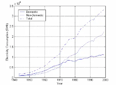
The electricity consumption for each of the three sets are shown in Figure 1. There is an increase in trend in the consumption data for all the sectors. However, the rate of consumption growth is generally very slow in the Domestic sector especially from 1975 onwards.

Figure 1: Electricity Consumption for the Various Data Sets.

3.3. AUTOCORRELATION ANALYSIS

The autocorrelation coefficients range from 0 to 1. When the correlation coefficients are high, i.e. close to 1, it implies that the data points are closely correlated at a certain time period. This means that it is statistically significant to make a forecast to the next time period

based on the present data. A summary of the rk values for time lags of k =1, 5, 10 and 15

years is given in Table 1.

Table 1: Autocorrelation coefficients for the Domestic, Non-Domestic and Total Data Sets

k =1 k =5 k=10 k=15

Domestic 0.9774 0.8832 0.7612 0.6389

Non-Domestic 0.9627 0.8264 0.6594 0.4910

Total 0.9695 0.8483 0.7008 0.5531

Sector

Autocorrelation Coefficient, rk

While there is a decrease in the value of autocorrelation coefficients for an increase in time lag, the coefficients for all the data sets indicates that they are high even at the 15 year lag. Thus, forecasting using time trend extrapolation of the present data can be applied as there is significant autocorrelation in the consumption data.

4. Logistic Curve Fitting

4.1. ESTIMATING THE UPPER LIMIT

Fitting the Logistic Curve is very dependent on the asymptote F obtained. Skiadas,

Papayannakis and Mourelatos [3] concluded that the saturation level is the most critical factor for understanding the behaviour of the system to which the Logistic Curve is to be applied. In this research F is obtained by regression analysis of the electricity consumption data concerned. This method should only be applied if the growth of development is at the latter stages [1]. The early development is strongly influenced by problems associated with immature technologies and should not be used to predict the maturity of a technology.

4.2. APPLICATION TO THE HISTORICAL DATA

The Fibonacci Search Technique is applied to all the three sets of electricity consumption data. A Matlab program has been developed that performs the Fibonacci search technique and produces the required results. The accuracy of the program was verified by comparing it to results previously obtained [1, 2].

Asymptotic values have been calculated for the entire sets of historical data available from 1943 to 1999. Table 2 shows the values of the asymptotes and the corresponding SSR values.

Table 2: Asymptotes F and the corresponding SSR values for the Logistic curve fitting using the Fibonacci search technique.

Sector Data Year F (GWh) SSR

Domestic 1943 - 1999 11420 6.4696E+06

Non-Domestic 1943 - 1999 24573 1.1922E+07

Total 1943 - 1999 36563 1.8670E+07

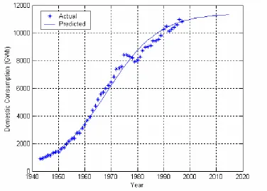
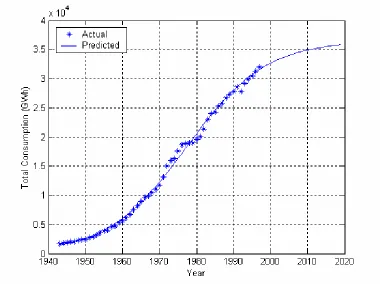
The Logistic curves obtained for the Domestic, Non-Domestic and Total sets of data are shown in Figure 2, Figure 3 and Figure 4 respectively.

Figure 3: Logistic Curve obtained for Non-Domestic consumption using Fibonacci search technique (F=24573 GWh).

When Tay [1] applied the Fibonacci search technique for data from 1943 -1981, the asymptote for the Non-Domestic sector (F= 41621 GWh) was greater than that for the Total Consumption (F = 32452 GWh). He came up with two possible explanations for this result. The first was that it might have been the effect of the inclusion of the electricity-intensive industries in the Non-Domestic consumption data, the second being that the consumption has not gone beyond the early stage far enough for a reliable Fibonacci optimal search to be applied. The calculation of the asymptotes in Table 2 shows that the asymptote for the Non-Domestic sector is below that for the Total consumption. This is a clear indication that the Non-Domestic sector has gone beyond the early stage of development, and thus the second explanation seems to be appropriate. Moreover the aggregated sum of the Domestic and Non-Domestic sector’s asymptotes is 35993. This is within 2% of the asymptote calculated for the Total consumption and indicates that both sectors and the total are well beyond the early stages of development and reaching maturity.

5. Comparison of Forecasts

5.1. COMPARISON OF HISTORICAL FORECASTS WITH ACTUAL

CONSUMPTION DATA

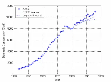
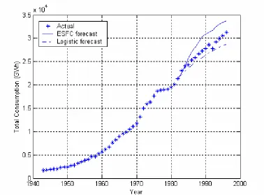
This section compares the forecasts made in 1982 by the Electricity Sector Forecasting Committee (ESFC) of New Zealand Electricity with the Logistic model forecasts [1, 2]. Since the actual consumption data is now available, these forecasts are compared with the actual data that has subsequently been accrued. All the forecasts are obtained for 15 years ahead assuming that the last known set of data available was for 1981. Figures 5 to 7 show the actual consumption data along with the ESFC forecast and the Logistic forecast for the Domestic and Non-Domestic sectors and the Total consumption respectively. Figures 8 to 10 show the percentage variation of the two forecasting methods from the actual data for the three sectors.

For the Domestic sector, the two sets of forecasts have underestimated the actual consumption over the entire forecast period. The Logistic Model has given a better forecast for the initial 6 years, but the variation in error has increased more than that for the ESFC forecasts for the longer term forecasts. For the Non-Domestic sector, both the sets of forecasts have overestimated the actual consumption. The Logistic forecast has generally given a closer estimate than the ESFC forecast, but both show significant departures from what has occurred. The electrification of commerce and industry has not proceeded at the rates predicted at that time.

Figure 5: Comparison of forecasts for Domestic Consumption

Figure 7: Comparison of forecasts for the Total Sector

Figure 9: Percentage variation of the forecasts from the Non-Domestic data

5.2: COMPARISON OF RECENT FORECASTS

5.2.1: AVAILABLE MODELS AND THEIR ASSUMPTIONS

Currently there are two sources of forecasts that are available for electricity consumption in New Zealand. Predictions are made by the Ministry of Economic Development (MED)[13] and another set of forecasts are published jointly by Sinclair Knight Merz and Centre for Advanced Engineering (CAE) [14].

The MED forecasts are made by the Energy Modelling and Statistics Unit of the Ministry of Commerce (Now Ministry of Economic Development), using its SADEM energy supply and demand model. The SADEM model is a descriptive market equilibrium model focusing on the entire energy sector. The model determines equilibrium in the energy market by projecting demands for a given set of prices and comparing this with the modelled cost of supplying this level of demand [13]. These demands are re-estimated if the prices implied by modelling the level of supply are not consistent with the prices used to determine the initial demand. The process of re-estimation is continued until equilibrium is achieved with demand and supply in balance at market clearing prices. An interpolation technique is used for updates of the prices. Thus, the forecasts are also interpolated between these dates.

The CAE forecasts are modelled using an annual load growth of 1.8%. Their study has used 1.8% as the baseline estimate, with 1.3% and 2.3 % growth used for sensitivity analysis. This report uses the 1.8% baseline estimate for comparison purposes with the Logistic model forecasts.

5.2.2: COMPARISON OF FORECASTS TO 2017

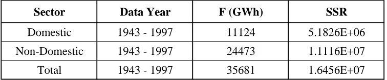
The MED and CAE forecasts are made using 1998 March year as the last set of known historical data. Therefore, Logistic model forecasts are obtained using the same set of historical data. Thus new values of asymptotes are obtained and Table 2 is updated as required and is illustrated in Table 3.

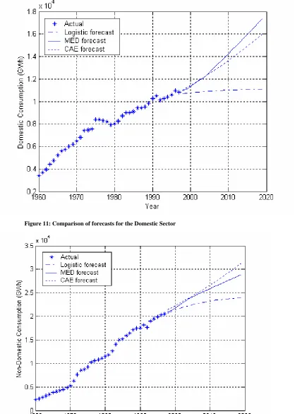
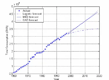
Figures 11, 12 and 13 shows the Logistic forecast, MED forecast and CAE forecast for the Domestic and Non-Domestic sectors and the Total consumption respectively.

Table 3: Updated Logistic model asymptote values for comparison of forecasts

Sector Data Year F (GWh) SSR

Domestic 1943 - 1997 11124 5.1826E+06

Non-Domestic 1943 - 1997 24473 1.1116E+07

Total 1943 - 1997 35681 1.6456E+07

Figure 11: Comparison of forecasts for the Domestic Sector

Figure 13: Comparison of forecasts for the Total consumption

As seen from the Figures, there are a number of variations in the forecasts. For the Domestic sector, the Logistic forecast is considerably below that for the other forecasting methods. While the MED and CAE forecasts assume a continuous growth, the Logistic forecast assumes a saturation of the consumption data. The difference is attributable to the assumption of inherent saturation or limits to growth that the logistic curve models, as against the unconstrained constant percentage growth assumptions in both the MED and CAE models.

For the Non-Domestic sector, forecasts are closer to each other than for the Domestic sector. The MED and CAE forecasting lines are higher than the Logistic model forecast again reflecting the inherent assumptions of limits or unconstrained growth for the various models. The CAE and MED model calculates the Non-Domestic sector consumption as the difference of the Total and Domestic consumption while the Logistic model is obtained directly by applying the Non-Domestic historical data. The rate of growth in the Logistic model is faster than for the Domestic sector. This indicates that there is a stronger demand for electrification in the industrial and commercial sectors than by residential customers. A similar trend is observed for the Total consumption in Figure 13. The CAE and MED forecasts are very similar while the Logistic model is predicting much lower consumption overall.

electricity is limited and that some form of substitution for electricity by another energy form may be required to sustain economic growth.

6. Effect of Historical Data on the Asymptotic Value

The asymptote of the Logistic Equation (3) has a significant effect on the forecasts made. Once the historical data is used to get the best fit, i.e, to get the constants of the regression equation, it is the upper limit, F, that determines the accuracy of the forecast. While, the Fibonacci Search Technique used to get the upper asymptote has been proven to be an effective method [1] the value of F will depend on the extent of the data used in determining it.

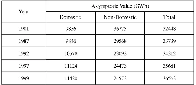
Asymptotic values are generated for the Domestic and Non-Domestic sectors and Total consumption with data values used up to a particular year. For each of the asymptotic values obtained, the base year is 1943. Thus, the asymptotic value for year 1987 is the asymptotic value obtained by the Fibonacci Search Technique for the years 1943 – 1987. Table 4 shows the asymptotic values for obtained for a number of selected years.

The year 1981 was chosen as this represents the extent of data available in previous studies [1, 2]. The year 1987 was chosen as this was the year that marked the introduction of deregulation of the electricity industry in New Zealand. The subsequent years of 1992, 1997 are at 5 year intervals and 1999 is the extent of reliable historical data.

Table 4: Asymptotes for Domestic, Non-Domestic and Total Sectors

Domestic Non-Domestic Total

1981 9836 36775 32448

1987 9846 29568 33739

1992 10578 23092 34312

1997 11124 24473 35681

1999 11420 24573 36563

Asymptotic Value (GWh) Year

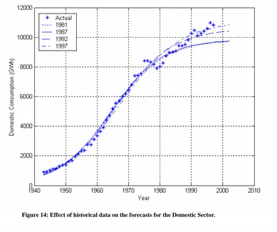
Figure 14: Effect of historical data on the forecasts for the Domestic Sector.

Figure 16: Forecasting lines for the Total Consumption.

From Figure 14, for the Domestic sector, the forecasts for 1981 and 1987 are very similar. Increasing the historical data used has given very comparable forecasts for subsequent years. As the extent of the historical data used increases beyond 1987, the forecasting lines increase in value. This is a direct result of the actual increase in Domestic consumption in these more recent years. This is an indication that a new factor has influenced the pattern of Domestic electricity consumption since 1987, and that this factor may well be the deregulation of the electrical industry. The response has been an increase in the electrification of homes.

The Non-Domestic Sector shows that it has yet not reached maturity in the initial forecasts. The high asymptotic value for 1981, which is even higher than that for the Total consumption, shows that Non-Domestic Sector is in its early years of growth. As the amount of historical data available increases there is a consistent decrease in asymptote value. This is mirrored in the forecasting lines resulting in lower consumption values. The asymptote value for 1999 is higher than that for 1997. This indicates that the Non-Domestic Sector has possibly reached its maturity as in the Domestic Sector. However, there is not enough data for this speculation to be conclusive.

In the forecasts for the Total consumption of Figure 16 there has been consistent increase in F for each of the consecutive 5 years. The resulting increase in the asymptote value is very small and there are very similar gap lengths separating the forecasting lines. This indicates that the Total consumption might be reaching maturity.

7. Conclusions

This paper has investigated the effectiveness of the Logistic growth curve model in predicting New Zealand electricity consumption. Earlier forecasts by the Electricity Sector Forecasting Committee of New Zealand (1982) were compared with the Logistic model predictions. For the Domestic sector, the Logistic Model had given a better forecast for the initial 6 years, but the variation in error had increased more than that for the ESFC forecasts for the longer term forecasts. For the Non-Domestic sector, both the sets of forecasts had overestimated the actual consumption indicating that electrification of commerce and industry has not proceeded at the rates predicted at that time. The forecasts for the Total consumption were more diverse. This was indicated by the fact that the ESFC model adopted the aggregate of the Domestic and Non-Domestic forecasts to get the Total consumption forecasts, while the Logistic model was fitted directly to the historical total consumption data. In general it could be concluded that the Logistic model forecasts had given rise to more accurate forecasts than those using economic data in.

Analysis was also made on the effect on the asymptotic value when the amount of historical data used is varied. This has revealed that there had been a significant effect on the asymptotes. For the Domestic sector and Total consumption, there had been generally a consistent increase in asymptotes every year implying that original predictions underestimated the continued growth of what could have been considered as sectors approaching maturity. For the Non-Domestic sector, the asymptote decreased as the amount of data used increases. This implies that this sector was initially immature but may now be approaching maturity. A more extensive analysis of other factors such as price change of electricity, general income or Gross Domestic Product (GDP) may now be required to explain these differences.

References:

1. Tay, H. S., Forecasting New Zealand Electricity Consumption, A report presented for

the degree of Master of Engineering, University of Canterbury, Christchurch, New Zealand, 1985

2. Bodger, P.S and Tay, H.S, Logistic and Energy Substitution Models for Electricity

Forecasting : A Comparison Using New Zealand Consumption Data, Technological Forecasting and Social Change 31,p 27-48, 1987

3. Skiadas, C.H, Papayannakis L.L. and Mourelatos, A. G, An Attempt to Improve

Forecasting Ability of Growth Functions: The Greek Electric System, Technological Forecasting and Social Change 44, p 391 – 404, 1993

4. Sharp, J.A. and Price, H.R., Experience Curve Models in the Electricity Supply

Industry, International Journal of Forecasting 6, 531 – 540, 1990

6. Tingyan, X., A Combined Growth Model for Trend Forecasts, Technological Forecasting and Social Change 38, 175 -186, 1990

7. Pearl, R., Studies in Human Biology, Baltimore Williams & Wilkins Company, 1924

8. Fisher, J.C. & Pry, R.H., A simple substitution of Technological Change, Tech.

Forecast & Social Change 3, 75-88, 1971

9. Mansfield, E., Technical Change and the Rate of Imitation, Econometrica, Vol. 29,

No. 4, 741 – 765, October 1961

10.Ministry of Energy, Electricity Forecasting and Planning: A Background Report to

the 1984 Energy Plan, 1982 -1984 issues

11.Ministry of Economic Development, New Zealand Energy Data File, July 2002

12.Boas, A.H., Modern Mathematical Tools for Optimisation, Part 3, Chemical

Engineering 105 -108, February 4, 1963

13.Ministry of Economic Development, Modelling and Statistics Unit, New Zealand

Energy Outlook to 2020, February 2000

14.Sinclair Knight Merz and CAE (Centre for Advanced Engineering, University of