Capacity Calculation and Sub-Optimal Power Allocation
Scheme for OFDM-Based Systems
Somnath Das, Abhishek Chakraborty, Sanjay Kumar Birla Institute of Technology, Mesra, India
Email: [email protected], [email protected], [email protected]
Received July 19, 2012; revised August 18, 2012; accepted September 21, 2012
ABSTRACT
For emerging cellular wireless systems, the mitigation of inter-cell interference is the key to achieve a high capacity and good user experience. This paper is devoted to the performance analysis of interference mitigation techniques for the downlink in an orthogonal frequency division multiple access (OFDMA) network, with a focus on the Long Term Evo-lution-Advanced (LTE-A) standard. Here we have derived a general closed-form equation of system capacity taking multiple cells into consideration and then we have investigated a coordination technique for interference mitigation. For the given interference constraint, how power should be transmitted into each OFDM sub-carrier for prevailing channel condition such that the total transmission rate of the base station can be maximized.
Keywords: Interference Reduction; LTE-A; OFDMA; Power Loading; System Capacity
1. Introduction
Radio spectrum is one of the most scarce and valuable resources for wireless communications. Given this fact, new insights into the use of spectrum have challenged the traditional approaches to spectrum management. LTE-A system with OFDMA as downlink multiple access tech-nique will have no intra-cell interference but will have a larger Inter-Cell Interference (ICI). Specifically, in [1] the authors have shown that OFDMA causes inter-cell interference among the users. The amount of interference introduced to the users by adjacent base station depends on the power allocated to the subcarrier as well as the spectral distance between particular subcarrier .The cell edge users are adversely affected due this ICI [2]. 3 GPP has proposed three different solutions to combat ICI i.e. randomization, cancellation and co-ordination, to counter this ICI problem [3]. An intelligent radio resource man-agement is needed for the dynamic allocation of radio resource to its users so as to maintain the QoS and also to best utilize the available spectrum while considering maximization of system throughput and capacity. Trans-mitter power control is an efficient technique to mitigate the effect of interference specially co-channels interfe- rence. Thus, an effective power control algorithms can offer a significant improvement in the system throughput. As we know that OFDM sub-carriers have time-varying fading gains, various power loading schemes have been proposed in the literature [4]. These algorithms maximize the transmission capacity of a single cell scenario. But
the use of classical loading algorithms e.g., uniform power and water-filling algorithms, for multi-cellular sce- nario may result in higher interference since, there exists no coordination. In this paper a downlink transmission has been considered in a multi-cell scenario. Hence, the design problem is as follows. Under interference con-straint, how much power should be transmitted into each OFDM sub-carrier for prevailing channels condition such that the total transmission rate of the base station can be maximized?
The organization of this paper is as follows. Section 2 gives a closed-form expression of system capacity for multi-cellular scenario. In Section 3, the system model is described. In Section 4, a suboptimal scheme has been proposed. In Section 5, numerical results are presented. Finally, Section 6 concludes the paper.
2. Closed-Form Expression of System
Capacity
From the context of information theory, for M number of adjacent cells closely spaced and N number of nodes in the target cell—the normalized (with respect to band-width) system capacity or spectral efficiency can be ex-pressed as
2
2 2
1 1 0
log 1
N M
n n
n m n m
p x C
N p h
p
n
(1)
where n is the delivered power to each sub-channel, N0 is the noise spectral density, x is the sub-channel
gain of the cell under consideration, and hm is the sub-
channel gain associated with the adjacent sub-channels and thus the term n m act as inter-cell interference to
the system. To maximize the system capacity, we have to maximize the above expression. So, in order to calculate the maximized system capacity, along with the Ka- rush-Kuhn-Tucker (KKT) conditions, the problem is de- scribed as follows
2 p h 2 2 0 n n n m p x
N p h
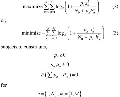
2 1 1 maximize log 1
N M
n m
(2)or,
2 2 0 nimize log 1
N M
n n
n m n m
p x
N p h
0 n p 0 n n p 2 1 1mi (3)
subjects to constraints,
pnPx
0
,m 1,M
0,
for
1,n N
The above constraints are self explaining. Here δ is the dual variable and μ is the slack variable. KKT holds for strong duality, which can be solved for two different ways but having equivalent solutions. Here
n 0
are called Lagrange’s multipliers or dual vari-ables. These KKT conditions are necessary and sufficient conditions for duality.
Now, taking the problem equation together with the KKT conditions, the partial Lagrangian equation is for-mulated as,
2 2 0 1 1 n n n m N N n n n n p xN p h
p
2 1 1 , , log 1 n n N M n m n x L p p P
(4)To calculate the maximum capacity based on the above expression, partial derivatives of the Lagrangian function with respect to Pn has to be taken and by
apply-ing KKT condition, the resultapply-ing equation becomes
1 ln 2
mn Y n m n p X
(5)
where,
2
0
1 n m
m n p h N X 2 2 0 2 0 n m m n n
N p h
Y
N x
From the above equation, the optimal power has to be calculated and thus the derived closed-form expression of optimized system capacity is given by
2
2
1 1 2
0 1 1 ln 2 log 1 1 1 ln 2 mn n N M mn mn
n m mn
m mn mn Y x X X C Y N h X X
1 k K
(6)
This is a generalized closed-form expression of system capacity for multiple cells scenario.
3. System Model
Here we have considered a two-cell scenario. Each cell uses OFDMA and hence, uses frequency reuse factor 1. The available bandwidth is divided into k subcarriers, where k ranges from
j J
i I
. It is assumed that the bandwidth for each sub-carrier is Hz and each user uses only one sub-carrier. The numbers of users under BS1 are j, where j ranges from 1 and users under BS2 are i, where i range from 1 . xbs j1, and
2,
bs i
x is the transmitted power of BS1 and BS2 respec- tively.
In downlink transmission scenario shown in Figure 1, there are four channel gains: i) between the BS2 and its
ith
user for the sub-carrier denoted as ii) between the BS2 and jth BS1 user, denoted as i iii) between
the BS1 and the ith BS2 user, denoted as i iv) be-
tween the BS1 and its jth user for sub-carrier denoted as
i The received signal at the receiver of jth user of BS1
and ith user of BS2 are and respectively
22 i h 21 h 11 h 11 h 1, bs j
y ybs2,j
11 21
1, 1, 2, 1,
1
I
bs j bs j j bs i j bs j
i
y x h x h n
22 12
2, 2, 1, 2,
1
J
bs i bs i i bs j i bs i
j
y x h x h n
1,
bs j
n nbs i2,
(7)
(8)
where and are the received noise at BS1
[image:2.595.55.291.188.379.2]22 i h 21 i h 12 i h 11 i h 1, bs j x 2, bs j x 2, bs j y 1, bs j y 1, bs j n 2, bs j n
and BS2 respectively. For protection of BS1 users, we consider constrains on the interference introduced by BS2. The total interference introduced to BS1 can be written as
1, 2, ,
j J
21
2, th
1
I
bs i j i
p h I
(9)4. Proposed Sub-Optimal Scheme
Considering this fact that most of the interference intro-duced to the BS1 users is inintro-duced by BS2 transmission over same sub-carriers. The problem can be formulated as follows
22
2 1 i i
i p h
1, 2, ,K
1 j I i T i p p
1, 2, ,
j K
i
12 1, 1
I
bs i j i
p h
1: max log2
j i I i I p P
(10)subject to
21 th 1
1, 2, ,
j I
i j i
p h I j J
(11)(12)
0 1, 2, ,
i
P i I
22
h
(13)
where is the channel gain from BS1 to its user and
2 2 AWGN i 2 (14)
AWGN is the mean variance of the additive white
Gaus-sian noise (AWGN). The interference is assumed to be the superposition of large number of independent com-ponents; hence, we can model the interference as Gaus-sian. Assuming that each carrier band is narrow, sub-carriers can be approximated as channel having flat and constant gains during transmission. K denotes the total no of sub-carriers, I is the no users of BS2 users and J is the no users of BS1 users. Ith denotes the interference thresh-old prescribed by the BS1 users. Interference threshthresh-old is the maximum tolerable interference on the spectrum be-ing utilized. It is highly variable dependbe-ing on the alloca-tion of channels to the users within the cell. However for simplicity we can assume a common threshold for all the channels. PT is the fixed total power budget of the sys-
tem. Ijdenotes the set of the same sub-carriers belonging
to the BS1. Using the same derivation in [5], we get
2 2 22 i i h 21 1 1 i J j j j p h
(15)where αand βare the non-negative dual variables corre-
sponding to the interference and power constraints re-spectively. The solution of the problem still has high computational complexity which encourages us to find a simpler, faster and efficient power allocation algorithm. The scheme proposed in this section is based on the fact that if the interference constraints are ignored in P1, the
solution of the problem will follow the well-known Wa-terfilling interpretation [6].
2 2 22 T P i i i p h
(16)
where λ is the waterfilling level and is given by
2 2 22 1 I i T i i P h
(17)On the other side, if the total power constraint is ig-nored, the Lagrangian of the problem can be written as [7] 2 22 2 2 1 21 1 1 log 1 Int I i i Int i i J I Int th j i i j i p h G I p h
(18)where is j the Lagrange multiplier. Equating
d d Int Int i G p
to zero, we get
2 2 21 22 1 Int i i Int j j i p h h (19) Int j
where value of
21
1 j I Int i th i i
can be calculated by substituting Equation (19) into
p h
I to get 21 2 2 22 j j Int j j i thi I i
I h I h
(20)
In order to solve the optimization problem P1, we can
start by assuming that the maximum power that can be allocated for a given subcarrier i is determined
ac-cording to the interference constraints only by using Equations (11) and (12) for every set of sub-carriers. By such an assumption, we can guarantee that the interfe-
n p
rence introduced to BS1 users will be under the pre-
o specified threshold. Once the maximum power pin is
determined the total power constrain is tested. If the t tal power constrain is satisfied, then the solution has been found and is equal to maximum power that can be allo-cated to each subcarrier, i.e. pi pin. Otherwise, the
available power budget should be buted among the subcarriers giving that the power allocated to each sub-carrier is lower than or equal to the maximum power that can be allocated to each subcarrier pin, and hence the
following problem should be solved: distri
22 2
1 i i
i h
(21)
subject to
WF T P
2 2
P
1
: max lo
i p
i1
j I
i p
g
i
j WF
I p
0
(22)
max
i i
p p
(23)
max
p
max
p
max
i p
WF
p pmax
WF p
max
WF
p p
WF
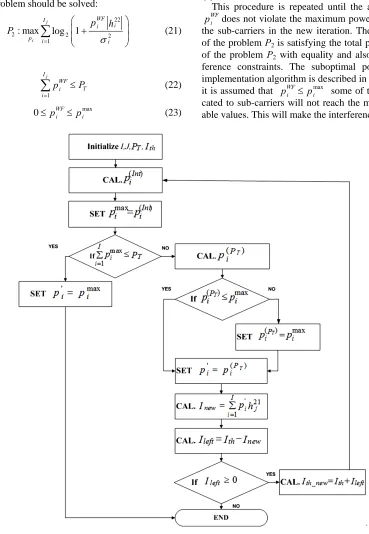
The problem can be solved efficiently using the con- cept of the conventional waterfilling. Given the initial waterfilling solution, the channels that violate the maxi- mum power i are determined and upper bounded with i . The total power budget is reduced by sub- tracting the power assigned so far. At the next step, the algorithm proceeds to successive water-filling over the sub-carriers that did not violate the maximum power
in the last step.
This procedure is repeated until the allocated power
i does not violate the maximum power i in any of
the sub-carriers in the new iteration. The solution i of the problem P2 is satisfying the total power constraint
of the problem P2 with equality and also satisfies inter-
[image:4.595.106.475.193.727.2]ference constraints. The suboptimal power allocation implementation algorithm is described in Figure 2. Since it is assumed that i i some of the powers allo- cated to sub-carriers will not reach the maximum allow- able values. This will make the interference introduced to
e BS1 user below t e threshold th
th h I . It is im
l
portant to mention that the power allocation po icy is indeed a wa- terfilling policy. However, the cut-off value for the chan- nel gain or the threshold for this waterfilling policy is weighted by the inverse of the interference term Ith. Specifically, the policy suggests that more power sho d be allocated to the sub-carrier which has relatively better channel quality.
ul
5. Results
presented in this section, we assume the In the results
values of I and J to be 20 and 4, respectively. We assume the value of total available bandwidth as 1MHz and no of subcarriers to be 33. The value of i is assumed to be
10–11 watts. The total power is assum d to be 10–3 watts. In Figure 3, we plot the achievable transmission rate of the BS2 versus interference threshold prescribed by BS1. The scheme tries to maximize the total throughput of the system under the constraint that each base station cannot
e
ore than a specific value PT and the introduc-
e plotted the interference intro-du
ed the transmit power and 1/
transmit m
ed interference to the neighbouring cell is within the in-terference threshold Ith.
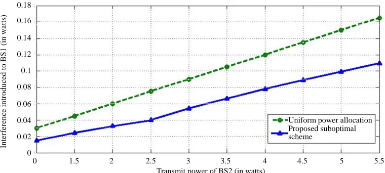
In Figure 4, we hav
ced to BS1 versus the transmit power of BS2. From this figure, we observe that for the same introduced in-terference level the proposed suboptimal scheme allows transmission of more power than the classical method like uniform power loading. This is possible because the suboptimal scheme considers the interference introduced to BS1 as one of its constraint. So there exists a harmony in power allocation over the sub-carriers which minimize the intercellular interference.
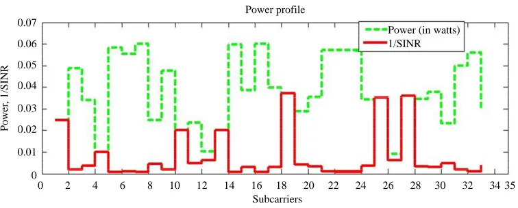
In Figure 5, we have plott
SINR for individual sub-carriers of BS2. 1/SINR basi- cally, represents the amount of interference present in the channel. The suboptimal scheme allows transmission of higher power over sub-carriers where the channel condi-tions are good and restricts power over sub-carriers where the channel conditions are bad.
Proposed suboptimal scheme Uniform power loading
0 0.015 0.03 0.045 0.06 0.075 0.09 0.105 0.12 0.135 0.15 0.16 Interference threshold (in watts)
×107
1.7
1.6
1.5
1.4
1.3
1.2
1.1
1
T
rans
m
issi
on r
ate
of
BS2 (
[image:5.595.109.488.344.514.2]in bps)
Figure 3. Interference introduced to BS1 vs. transmit power of BS2.
Uniform power Proposed subo scheme
allocation ptimal
0 1.5 2 2.5 3 3.5 4 4.5 Transmit power of BS2 (in watts)
5 5.5 0.18
0.16 0.14 0.12 0.1 0.08 0.06 0.04 0.02 0
Inte
rfe
re
nc
e in
tro
d
u
ce
d
to B
Figure 4. Transmission rate of BS2 vs. interference introduced to BS1.
S1
(in
wa
tts)
[image:5.595.104.484.545.716.2]Power (in 1/SINR
watts)
0 2 4 6 8 10 12 14 16 18 20 22 24 26 28
Subcarriers
30 32 34 35
0.07
0.06
0.05
0.04
0.03
0.02
0.01
0
Power
, 1/SI
N
R
[image:6.595.110.488.82.234.2]Power profile
Figure 5. Power profile.
ave developed a suboptimal power
sightful comments of Md
[1] T. Weiss, J. and F. K. Jondral,
tion—White Paper,” 2008.
logy/whitepapers/lte_ove
au, J. Panicker, N. Guo, R. Chang, N. Wang
6. Conclusion
In this paper, we h
loading algorithm that maximizes the downlink transmis-sion data rate of the BS2 while the interference intro-duced to the BS1 user remains within a given limit. The proposed algorithm is simpler and more efficient in terms of throughput performance.
7. Acknowledgements
Authors acknowledge the in . Irfanul Hasan, Research scholar, B. I. T., Mesra, Ranchi, India.
REFERENCES
Hillenbrand, A. Krohn
“Mutual Interference in OFDM-Based Spectrum Pooling Systems,” Proceeding of IEEE Vehicular Technology Con- ference (VTC’04), Milan, 17-19 May 2004, pp. 1873-1877.
[2] Ericsson, “Long Term Evolution (LTE): An Introduc-
http://www.ericsson.com/techno rview.pdf
[3] G. Boudre
and S. V. Nortel, “Interference Coordination and Cancel- lation for 4G Networks,” IEEE Communications Maga- zine, Vol. 47, No. 4, 2009, pp. 74-81.
doi:10.1109/MCOM.2009.4907410
[4] A. Leke and J. Cioffi, “A Maximum Rate Loading Algo-
Hossain and V. K. Bhargava, “Adaptive
rce Allocation for OFDM-Based Cog-
ptimization,” Cam- rithm for Discrete Multi-Tone Modulation Systems,” Pro- ceedings of the IEEE Global Telecommunications Con- ference (GLOBECOM’97), Phoenix, 3-8 November 1997, pp. 1514-1518.
[5] G. Bansal, M. J.
Power Loading for OFDM-Based Cognitive Radio Sys- tems,” IEEE Communications Magazine, Vol. 46, No. 9, 2008, pp. 59-67.
[6] Y. Zhang, “Resou
nitive Radio Systems,” Ph.D. Dissertation, University of British Columbia, Vancouver, 2008.