FOR
POWER SYSTEMS
A thesis presented for the degree of
Doctor of Philosophy in Electrical Engineering
in the
University of Canterbury,
New Zealand,
by
James Ranil de Silva, B.E.(Hons 1)
taos
Mostly for my father, the late
Abstract
This thesis extends the concept of the traditional synchronous
generator capability chart to describe the steady state performance of
transmission lines, HVOC links, and entire AC/OC power systems.
Each capability chart depicts an operating region on the complex
power plane that represents the real and reactive power that may be
supplied to a load from a particular busbar. The boundaries of the
operating region are defined by a web of contours that represent the
critical operating constraints of the system.
The charts for small systems can be constructed by manipulating the
operating equations into a form suitable for drawing loci on the complex
power plane. This technique is used in this thesis to construct charts
for generators, transmission lines, and HVOC links.
The operating equations of large systems are not easily manipulated,
so a different approach is used to construct charts for large systems.
This approach involves iterative powerflows and contour plotting to avoid
the formulation of explicit closed form locus equations.
Two algorithms for drawing the capability charts of large AC power
systems are described. The first algorithm uses a contour tracing
technique to plot the constraint loci. The knowledge gained from the use
of this algorithm was then used to design the second, faster algorithm
that uses a region growing technique to help plot the constraint loci.
Capability charts for large AC/OC systems are also discussed. The
operating constraints of the AC/OC converters require special treatment
due to discontinuities in the converter operating equations. An offshoot
of the work on AC/OC charts is the development of an improved sequential
AC/OC powerflow algorithm.
A practical example of the use of the capability charting algorithms
is given by drawing charts for a proposed second New Zealand HVOC link.
The capability charting algorithms will make suitable additions to
existing power system interactive graphics programs. On-line displays of
capability charts in system control centres could also provide useful
List of Contents
Abstract
List of Contents
Acknowledgements
Page
(i)
(iii)
(viii )
(ix) Publications Associated with this Thesis
CHAPTER 1 INTROD~CTION
1.1 Graphics, Power Systems, and Capability Charts
1 .2 Historical Background
1
.3
Chapter ReviewCHAPTER 2 CHARTS FOR SIMPLE POWER SYSTEMS 6
2.1 Introduction 6
2.2 The Capability Chart for a Synchronous Generator 7
2.2.1 Simplifying Assumptions 8
2.2.2 Generator Vector Diagrams 8
2.2.3 Construction of the Capability Chart 13
Turbine Power Limits 13
Maximum Stator Current 13
Rotor Current Limits 1~
Steady State Stability Limit 14
2.2.4 Summary of Synchronous Generator Chart 18
2.3 The Capability Chart for a Transmission Line 18
2.3.1 Transmission Line Model 19
2.3.2 Operating Constraints 20
Load Busbar Voltage Limits 21
Voltage Stability 23
Maximum Transmission Line Current 26
2,3.3 Capability Chart on the Admittance Plane 29
Voltage Limits 30
Line Current Limit 30
2.3.4 Summary of Transmission Line Capability Charts 31
Page
CHAPTER 3 A CHART FOR AN HVDC LINK 33
3.1 Introduction 33
3.2 Circuit Model of the HVDC Link 33
3.3 Operating Constraints of the HVDC Link 38
Converter Transformer Current 38
Converter Valve Current 38
Harmonic Filter Current 38
DC Voltage Rating 39
Converter Control Angles 39
Converter Commutation Angle 39
Capability of the Benmore Generator 40
Interconnecting Transformer Current 41
3.4 Loci of Operating Constraints 41
3.4.1 AC/DC Per Unit System 41
3.4.2 Basic AC/DC Converter Operating Equations 42
3.4.3 Loci of Haywards Converter 43
Commutation Overlap Locus 44
Loci of DC Current Limits 44
Locus of Maximum Converter Transformer Current 46
Loci of Maximum DC Voltage 46
Locus of Minimum Firing Angle 47
Locus of Minimum Extinction Angle 47
3.4.4 Loci of Benmore Converter 48
DC Link Power Transfer Mapping 48
3.4.5 Loci of South Island Power Generation 50
3.4.6 Complete Capability Chart 52
Page
CHAPTER ~ CHARTS FOR LARGE AC SYSTEMS
56
~.1 Introduction
56
~.2 System Operating Constraints 57
~.2.1 Voltages and Currents on Transmission Lines 58
~.2.2 Generator Capability 58
~.2.3 Steady State Stability 58
~.2.~ Total Constraint Number 59
~.3 Test System 59
~.~ Capability Charting Algorithm 62
~.~.1 Definition of the Vicinity of the Operating
Region 62
~.~.2 Structure of the Capability Charting Algorithm 63
System Data Input 63
Seed Point
66
Search for Vicinity Perimeter 66
Contour Following Algorithm 67
Tracing of Constraint Contours 70
~.~.3 Interpretation of Capability Chart 71
~.~.~ Holes and Islands 7~
~.~.5 Shortened Labels for Diagram Dressing 76
~.5 Conclusion 76
CHAPTER 5 A FAST CAPABILITY CHARTING ALGORITHM 78
5.1 Introduction 78
5.2 Structure of the Fast Algorithm 79
5.2.1 Region Growing 80
5.2.2 Contour Plotting 82
5.3 Powerflow Convergence Boundary 86
5.~ Contour Maps 88
CHAPTER
6
CHARTS FOR LARGE AC/DC SYSTEMS 6.1 Introduction6.2 Operating Constraints of DC systems
6.2.1 Constraints of DC Rectifier
6.2.2 Constraints of HVDC Link
Page
91
91
91
92
92
6.2.3 Allow~ble Range of Values for DC system Variables 94
6.3 Improving the Sequential AC/DC Power flow 96
6.3.1 Conventional Sequential Powerflow 97
6.3.2 Improving the Sequential Powerflow 97
6.3.3 Comparison of Convergence Behaviour 99
6.4 AC/DC System Capability Charts 104
6.5 Conclusion 108
CHAPTER 7 PLANNING FOR A SECOND N. Z. HVDC LINK 109
7 . 1 Introduction 109
7.2 South Island Terminal 110
7.2.1 Capability Chart for Bendigo Converter Busbar 112
7.2.2 Capability Chart for Ohau A Generator Busbar 114
7.2.3 Voltage Fluctuations at the Bendigo Converter
Busbar 11 6
7.3 North Island Terminal 118
7.3.1 Capability Chart for Runciman Converter Busbar 120
7.3.2 Capability Chart for Huntly Generator Busbar 122
Page
CHAPTER 8 PROPOSED DEVELOPMENTS 125
8.1 Introduction 125
8.2 More Detailed Models 125
8.3 Generation Cost Contours 126
8.4 Optimal Powerflow Algorithms 127
8.5 Stochastic Power flow Algorithms 127
8.6 Eigenvalue Representation 128
8.7 Interactive Graphics Programs 130
8.8 System Control Applications 131
8.9 Conclusion 134
CHAPTER 9 MAIN CONCLUSIONS 135
References 138
Appendix: C ircu i t Da ta 141
A1 IEEE 14 Busbar Test System 141
A2 HVDC Link Modification to IEEE 14 Busbar Test System 144
A3 New Zealand South Island Primary System 145
Acknowledgements
.My thanks to Dr Christopher P. Arnold for his supervision during the three years of research involved in this thesis.
I am also indebted to my employer, the Electricity Division of the
Ministry of Energy, who gave me leave to do the work.
Thanks to the staff and postgraduate students at Ilam, particularly
Bill Kennedy and Andrew Earl for the efforts they have put into the
computing and graphics facilities. Also Professor Josu Arrillaga, Dr
Patrick Bodger, Enrique Achadaza, Gordon Cameron, Neville Watson, and
Chris Callaghan for their discussions and humour.
Special thanks to my family who completely and utterly approve of
Publications Associated
with this Thesis
The following three publications are associated with the research
presented in this thesis.
Arnold, C.P., and de Silva, J.R., "A Capability Chart for Power
Systems", Second International Conference on Power System Monitoring and
Control, Durham, UK, 1986.
de Silva, J.R., and Arnold, C.P., "Capability Charts for Analyzing Power
Systems", to be presented at the Conference of the Insti tute of
Professional Engineers New Zealand (IPENZ), 1987.
de Silva,
Chart for
J.R., Arnold, C.P., and Arrillaga, J., "A Capability
an HVDC Link", accepted for publication in the lEE
Proceedings-C Generation, Transmission, and Distribution, 1987.
The following paper has also been submitted for publication but has
yet to be officially accepted (as of 11th March, 1987).
de Silva, J.R., and Arnold, C.P., "A Simple Improvement to Sequential
AC/DC Power flow Algorithms", submitted to the Electric Energy Systems
Introduction
1.1 GRAPHICS, POWER SYSTEMS, AND CAPABILITY CHARTS
An old adage that claims "A picture paints a thousand words" conveys
the essence of graphical presentation. A good diagram can be more easily
understood than many pages of writing and, in particular, a good graph is
preferable to tables of technical data. The appeal of graphical displays
has grown as computer based graphics systems have progressively reduced
the labour required to produce an effective display. The blossoming
popularity of computer graphics is being reflected in the field of power
systems as more research effort is commi tted to the development of
graphics software specifically for power system analysis.
The best example~ of the use of computer graphics for analyzing power systems are the interacti ve graphics programs that have been recently
developed to model power system operation. Two such programs are IPSA
(Interactive Power Systems Analysis) described by Lynch and Efthymiadis
( 197 9) and ADAPOS (Advanced Analyzer of Power Systems) descri bed by
Fujiwara and Kohno (1985). These programs allow the user to interactively
construct a power system model by drawing the circui t diagram on a
graphi cs termi nal. Powerflow, transient stabili ty, and short circui t
studi es can then be performed wi th the resul ts appeari ng alongside the
circui t diagram.
Graphical displays of circuits are also commonly used in system
control centres to monitor the operation of the network. These displays
can be used interacti vely to directly control circui t breakers and
generators. More than a decade of use has proven that graphical displays
are beneficial for both modelling and monitoring power systems. Further
improvements in power system 'graphics can be expected from continued
research and development.
The particular development of power system graphics that is explored
in this thesis involves the drawing of capability charts. The capability
charts represent another method of graphically displaying power system
therefore related to other power systems graphics software and could be
profitably included in existing power system interactive graphics
packages.
The capability charts are drawn on the complex power plane and define
the real and reactive power that may be suppl ied from a bus bar during
steady state operation. The power available is depicted by a region on
the plane, the boundaries of the region represent the critical operating
limits of the system.
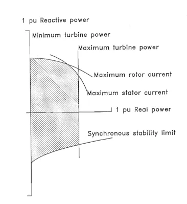
The best known example of a capability chart is the operating chart
of a synchronous generator as shown in figure 1.1 . The power available
from the generator is restricted by the rotor current, stator current,
turbine power, and synchronous stability limits. The work discussed in
this thesis can be considered to be a generalization of this concept of
a genera tor capabi li ty chart. This work can be placed in historical
context by considering the origins of capability charts.
1.2 HISTORICAL BACKGROUND
The origins of the power system capability charts lie with the power
circle diagrams that were introduced by Philip (1911) and later extended
by Evans and Sels (1921) and Dwight (1922). The circle diagrams provide a
graphical solution to the problem of relating the voltages and the real
and reactive powers associated with a transmission line. A compass and
ruler are the only tools required to construct the diagrams, providing
that the system studied is restricted to only a single transmission line.
This approach has proved to be very successful and is still used to solve
transmission line problems.
Szwander (1944) applied the circle diagram approach to drawing a
capabili ty chart for round rotor synchronous turbo-generators. Walker
(1953) later modified this chart to accommodate the characteristics of
salient pole generators. A simple equivalent circuit was used to model
the generators to simplify the derivation of equations and aid
construction of the chart.
1 pu Reactive power
Minimum turbine power
Maximum turbine power
Maximum rotor current
Maximum stator current
1 pu Real power
Synchronous stability limit
Figure 1.1 Capability Chart of a Synchronous Generator
The shaded operating region represents the real and
reactive power that may be supplied by the generator. The
boundaries of the region indicate the cri tical operating
[image:17.562.122.489.105.505.2]converters that were just beginning to proliferate at the time. Again a
simple system representation was used to simplify the circuit analysis.
All of the charts mentioned so far are restricted to describing
small, simple systems because the equations associated wi th each curve,
must be explicitly derived. If the curves can be shown to be circles or
other simple geometric shapes then the chart can be easily constructed.
If larger power systems are considered then the system equations rapidly
become much more complicated and prevent the simple derivation of
explicit curve .equations.
The use of iterative solutions to large power system equations avoids
the problem of formulating explicit derivations. A computer becomes
necessary to handle the calculation burden that is involved in the
iterative algorithms. A graphics output facility is also required to draw
curves that are much more complicated than the simple circle diagrams.
Wirth et al.
(1983)
used the iterative approach to draw contour maps of system eigenvalues on the complex power plane. These contour mapsdescribe the steady state stability of the power system. Price
(1984)
also used the iterative approach to draw a contour map of the powerflow
function for large systems on the complex power plane.
Price's work is probably the closest relative to the capability
charting algorithms that are described in this thesis. These algorithms
combine the contours associated with the most critical operating limits
to form capability charts for large power systems.
1.3
CHAPTER REVIEWThe discussion on capabili ty charts progresses from small, simple
systems to larger, more complicated networks. The capability charts of
two small systems are discussed in chapter 2. First the standard method
of constructing the chart for a synchronous generator is reviewed. A
modi f i cation of the circl e diagram approach is then used to draw the
The capability chart for an HVDC link is described in chapter
3.
A growing interest in HVDC links makes this chart particularly useful.The New Zealand Benmore-Haywards HVDC system is used as an example to
demonstrate the technique for drawing the chart.
The generator, transmission line, and HVDC link systems all have
small, specific configurations. An algorithm for drawing capability
charts for larger, general AC systems is described in chapter 4. This
algorithm uses an iterative powerflow solution to handle the large number
of system equations. The algorithm also incorporates a contour tracing
technique to draw the chart boundaries.
The experience gained from drawing a large numoer of capability
charts has suggested possible improvements to the original charting
algori thm described in chapter 4. These improvements are incorporated
into a fast capability charting algorithm that is described in chapter 5.
The fast algorithm uses a region growing procedure to plot the critical
operating curves in preference to the contour tracing technique used by
the original algorithm.
The capabili ty charts for large AC/DC systems are then examined in
chapter 6. The charting algorithms are modified to incorporate the
opera ting constraints of rectifiers and two terminal HVDC links. The
AC/DC systems are analyzed by a new sequential AC/DC powerflow algorithm
that converges to a solution faster than previous sequential algorithms.
Chapter 7 describes the application of capability charts to help
study a proposed second HVDC link between the North and South Islands
of New Zealand.
The future prospects of research into capability charts are examined
in chapter 8. More detailed modelling of the power system is envisaged to
allow a greater variety of operating limi ts to be portrayed on the
charts. Generation cost contour maps are suggested to help minimi ze
opera ting cos ts. Consideration is given to the possibili ty of using
optimal powerflows and stochastic powerflows wi thin the capabili ty
charting algorithms. The incorporation of capability charts into existing
power systems interactive graphics programs is also discussed. Finally,
the potential application of capability charts for system monitoring is
Chapter 2
Charts for Simple Power Systems
2.1 INTRODUCTION
The tradi tional capability chart for a synchronous generator was
introduced by Szwander (1944) to display the relationship between the
operating limits of a round rotor machine. The steady state operation of
a round rotor generator can be described by a few equations and modelled
by a simple equivalent circuit. The generator capability chart is easily
constructed by manipulating the operating equations into a suitable form
for drawing loci on the complex power plane.
The same approach can be used to construct the capability charts for
other simple power system circuits such as the transmission line chart
and the HVDC link chart that are also described in this thesis.
The operation of larger power systems is described by a large number
of equations that cannot be easily manipulated into a suitable form for
drawing loci. A different technique is used to construct the charts for
these systems and this is treated in chapters 4 to 7 of this thesis.
The capability charts of small, simple systems still retain a valuable
role that is not negated by the development of the algori thms to draw
charts for larger, more complicated networks. The charts associated with
large networks cannot offer the same insights that can be gained from the
explicit derivation of locus equations for small systems.
Many of the loci for small systems can be drawn by hand without the
assistance of a computer. If facilities are not available to implement
the programs for drawing charts for large systems then it may be
possible to model the system being studied by a simple equivalent
circuit that can be analyzed by hand.
This chapter describes the construction of 'capability charts for two
simpl e power systems. First the tradi tional chart for a synchronous
generator is reviewed then a chart is developed to, describe the
2.2 THE CAPABILITY CHART FOR A SYNCHRONOUS GENERATOR
The capability chart for a round rotor synchronous generator was originally developed by Szwander (1944). The concept was later extended by Walker (1953) to include the operation of salient pole synchronous generators . This section reviews the construction of a chart for a salient pole generator and regards the round rotor generator as a special case of salient pole machines.
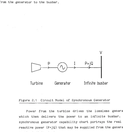
Figure 2.1 shows the ci rcui t model of a synchronous generator supplying power to an infinite bus bar • The purpose of the capability chart is to describe the range of complex power that may be delivered from the generator to the busbar.
v
P
I
Turbine
Generator
Infinite bus bar
Figure 2.1 Circuit Model of Synchronous Generator
[image:21.562.70.477.262.698.2]2.2.1 Simplifying Assumptions
To simplify the analysis the following assumptions have been made
1. The generator is connected to an infinite busbar. This is a strong
system that is able to maintain a constant voltage and frequency.
2. Only steady state operation is considered. All changes take longer
than the machine's transient time constant.
3.
Magnetic saturation is neglected. All inductive reactances in the model are therefore constant and independent of current.4. Losses due to hysteresis, eddy currents, and winding resistance are
neglected.
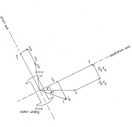
2.2.2,Generator Vector Diagrams
The vector diagram shown in figure 2.2 illustrates the relationship
between the voltage, current, and magnetic flux phasors of the generator.
The phasors have been superimposed onto a diagram representing the
position of the rotor and the position of the stator winding. The current
and flux phasors are resolved into components along the direct and
quadrature axes of the rotor. This resolution is necessary to deal with
the magnetic assymmetry of the salient pole rotor.
The rotor field current produces the flux Ff along the direct axis
of the rotor. This rotating flux varies sinusoidally at the stator
winding and induces the sinusoidal open circuit terminal voltage E. The
instantaneous value of E reaches a maximum when the vector Ff is cutting directly through the stator winding hence E lies along the quadrature axis.
The vector Ff may ~lternatively be regarded as a complex phasor that represents the component of flux passing perpendicularly through the
plane of the stator winding. The induced voltage E is equal to the time
derivative of Ff by Faraday's law. Therefore the sinusoidal flux Ff must lead the sinusoidal voltage E by 90 degrees, and E must lie along the
quadrature axis. This is in agreement with the previous argument based on
When the generator is loaded the stator current I lags the terminal
voltage V by the power factor angle rp. The current I can be resolved into
a direct axi s component Id and a quadrature axis component Iq
.
current Id produces a flux Fd that lies along the direct axis. current Iq produces a flux Fq that lies along the quadrature axis. and Fq are added to Ff to produce the effective rotating flux Fe .
\
\
\ \
~
000
stator
\-lirdingFigure 2.2 Vector Diagram of Salient Pole Synchronous Generator
The voltage, current, and magnetic flux phasors have been
superimposed on the rotor and the stator winding. The current
and flux phasors have been resolved into components along the
direct and quadrature axes of the rotor.
The
The
[image:23.562.73.513.195.617.2]The combined effect of Fd and Fq is called the 'armature reaction'
which tends to reduce the magnitude of Fe and lower the induced voltage
E. This can be conveniently simulated by one voltage drop due to Id
flowing through a direct axis armature reactance jXad and another voltage drop due to Iq flowing through a quadrature axis armature reactance jXaq •
In a sal i en t pole machine the direct axi s has a lower magnetic
reluctance path than the quadrature axis due to the larger air gap along
the quadrature axis. The value of jX ad is therefore larger than the value of jX aq • In a round rotor machine the reluctances of the two paths are almost identical and jXad is considered equal to jXaq .
The two components of the current I both flow through the stator leakage
reactance jXI • This reactance can be added to the armature reactances to form an effective direct axis reactance jXd and an effective quadrature axis reactance jX q .
'X
J q
'X +'X
J ad J I
jX +'X
aq J I
(2.2.2.1 )
(2.2.2.2)
The vectorial addition of the voltage drops jIdXd and jIqXq to the terminal voltage V produces the no load terminal voltage E. The angle 0
between V and E is called the rotor angle. This angle tends to increase
as more power is delivered from the generator.
Inspection of the vector diagram leads to the following steady state
operating equations that relate the magnitudes of the vectors.
Ivl·sin(o) I I I·X q q (2.2.2.3)
I V I . cos (0) lEI - IIdl,xd (2.2.2.4)
I I I . cos (</» I I I. cos (0) + IIdl·sin(o) (2.2.2.5)
q
III·sin(</» I I d I . cos (0) - II I·sin(o) (2.2.2.6)
It is convenient to directly relate E, V, and I without the use of
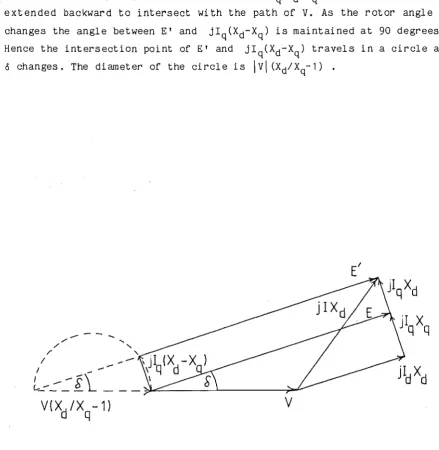
the orthogonal components Id and I q. To achieve this, the voltage vectors of figure 2.2 can be modified as shown in the vector diagram of figure 2.3 .
The voltage drop jIqXq has been extended to jIqXd so that the current I can be directly incorporated into the diagram as the voltage drop jIXd
The no load vpltage E is translated by jIq(Xd-Xq ) to E' and a line is extended backward to intersect with the path of V. As the rotor angle 0
changes the angle between E' and jIq(Xd-Xq ) is maintained at
90
degrees. Hence the intersection point of E' and jIq(Xd-Xq ) travels in a circle as<5 changes. The diameter of the circle is
Ivi
(Xd/Xq-1) •
, /
, /
I
--; 'v
Figure 2.3 Geometric Modification of Generator Voltage Vectors
The original generator vol tage vector diagram is modified to
[image:25.562.58.498.168.619.2]This geometrical manipulation serves to portray EI , V and jIX d as
part of a simple triangle. This triangle can be mapped onto the complex
power plane by imposing the following transformation on each vector A to
map it onto the corresponding vector AI on the complex power plane.
AI (2.2.2.7)
Where the symbol
*
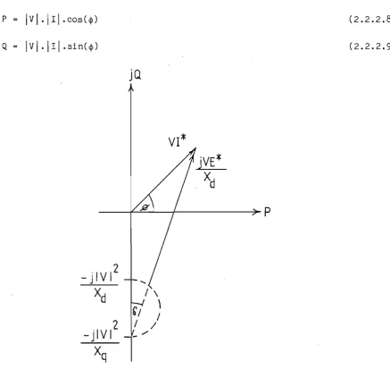
represents complex conjugation.The triangle on the complex power plane is shown in figure 2.4 . The
axes on the plane represent the real power P and the reactive power Q
that are delivered from the generator to the busbar.
P
Q
I V I . I I I . cos ( </> ) (2.2.2.8)
IVI·III·sin(</» (2.2.2.9)
jQ
VI*
--~=-....!...-+---30-p
_ j IV 12
Xd
I \\
~I I2
I /- jlV I
, /Xq
Figure 2.4 Generator Vector Diagram on the Complex Power Plane
The capability chart for the generator can be directly
[image:26.563.60.498.288.701.2]2.2.3 Construction of the Capability Chart
The vector diagram shown in figure 2.4 is in a suitable form for
easily constructing the capability chart of a salient pole generator. A
generator with the following specifications is used to demonstrate the
construction technique j
1. Turbine power range of 0 MW to 60 MW
2. Generator apparent power rating of 75 MVA
3. Excitation system capable of providing rotor field current
corresponding to a no load vol tage range of 0.1 to 2.0 pu
4. Direct axis reactance Xd
=
1.5 pu Quadrature axi s reactance X q = 1.1 pu5. Infinite busbar voltage V = 1 .0 pu
A 100 MVA power base is used for the per unit system.
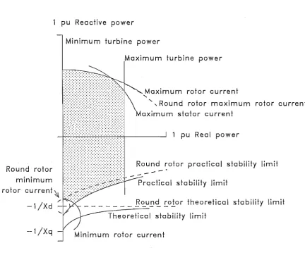
The capability chart is illustrated in figure 2.5 and depicts the
real and reacti ve power that can be supplied from the generator to the
infinite busbar. Each critical operating constraint is represented by a
s epar at e locus on the chart. The shaded area denotes the safe operating
region of the generator.
Turbine Power Limits
The generator has been assumed to be lossless so the entire turbine
power output is delivered to the infinite busbar. The maximum and minimum
turbine power limits are therefore represented as straight vertical lines
that intersect the real power axis at 0.0 pu and 0.6 pu •
Maximum stator Current
The apparent power rating of 75 MVA indicates that the stator current
I is limited to 0.75 pu to prevent overheating of the stator windings. If
I is fixed at this value the vector
vr*
in figure 2.4 traces out a circleof radius IVII centred on the origin. A small portion of this circle
contributes to the boundary of the operating region on the capabili ty
Rotor Current Limits
The upper limi t of the rotor field current is determined by the
heating of the field winding and the maximum current that can be
delivered by the, excitation system. The excitation system also imposes a
lower limi t on the rotor current. The no load termi nal vol tage E is
directly proportional to the field current i f magnetic saturation is
neglected. Therefore the upper and lower 1 imi ts of the rotor current
also correspond to upper and lower limits on the magnitude of E.
The loci that represent these limits are constructed by maintaining E
at its limiting value in figure 2.11 and varying the rotor angle
o.
The locus traced out byvr*
is in the shape of a slightly distorted circlecalled a 'Limacon of Pascal'.
On the capability chart the locus of maximum rotor current limits the
reacti ve power that can be generated and the locus of minimum rotor
current limits the reactive power that can be consumed at small leading
power factors.
If Xq is increased to the same value as Xd to simulate a similar
round rotor generator then the rotor current loci become circles centred
The locus of maximum rotor current for a round rotor
generator is almost indistinguishable from the locus of maximum rotor
current for a salient pole generator. The loci of minimum rotor current
are more easily distinguished because the effect of saliency is more
pronounced for small val ues of E.
Steady State Stability Limit
The steady state stability of a generator is determined by its
ability to respond to small disturbances without losing synchronism.
During these disturbances generators with slow acting exciters will
maintain a constant rotor current and a constant open circui t terminal
vol tage E. Under these condi tions the real power output P becomes
strongly dependent on the rotor angle
o.
The relationship between P and 0can be obtained by first substituting (2.2.2.5) into (2.2.2.8) to give
p
I
VI . [ I
II·
cos (0) +I
II.
si n (0) ]pu Reactive power
Minimum turbine power
Maximum turbine power
Maximum rotor current
...
... , Round rotor maximum rotor current
Round rotor minimum rotor current~
-1/Xd
,..
-l/Xq
Figure 2.5
Maximum stator current
1 pu Real power
Round rotor theoretical stability limit
~---Theoretical stability limit
Minimum rotor current
Capability Chart of a Salient Pole Generator
The chart portrays the real and reactive power that may
be supplied from the generator to the infinite busbar. The
shaded area denotes the safe operating region which is
bounded by loci that represent the critical operating limits
of the generator. The chart of a similar round rotor generator
differs in the positions of the rotor current and stability
loci. For comparison these round rotor loci are drawn on
[image:29.562.68.501.116.478.2]then substitution of Iq and Id from (2.2.2.3) and (2.2.2.4) gives
P
+
+ . co s (<') ) ] • sin (<') )
x
d
IvI2.(Xd- X ).sin(2.<') q .
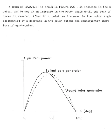
A graph of (2.2.3.2) is shown in figure 2.6 • An increase in the power output can be met by an increase in the rotor angle until the peak of the curve is reached. After this point an increase in the rotor angle is accompanied by a decrease in the power output and consequently there is a loss of synchronism.
1
pu Real powerSalient pole generator
I
I
o
I
I
I
I
I I
I
/' /
90
"
"-,
,
\
\
\Round rotor generator
,
, ,
o
(deg)180
[image:30.562.57.486.193.690.2]In a round rotor generator the second term of (2.2.3.2) is zero and
the corresponding power/rotor angle graph is sinusoidal. In this case
synchronism can be theoretically maintained until the rotor angle exceeds
90 degrees. The locus of the theoretical stClbili ty limit for a round
rotor generator is shown on the chart as a horizontal straight line
intersecting the reactive power axis at -1/X d •
The theoretical stability limi t for a salient pole generator is
obtained by differentiating (2.2.3.2) with respect to 0 to find the
maximum power output.
dP
Iv 1
.1
EI .
cos (0 )do
+
IvI
2.cOS(2.0).(Xd-X q )
Xd·Xq
This can then be solved .for cos(o).
cos(o)
-I
E1
•
Xq
+
[-I
v-:-~ :-~-:~-X-q
T
+ 8 4(2.2.3.3)
(2.2.3.4)
The locus of the theoretical stabili ty limit is drawn by gradually
varying E in (2.2.3.4) and obtaining the corresponding stability angle o.
The pairs of E and 0 values are then used in the vector diagram of figure
2.4 to obtain the corresponding points on the complex power plane.
The theoretical stability limit does not allow for a margin of safety
so a practical stability limit is defined. The practical limit allows for
a power increase of 10% of the turbine rating before the theoretical
limit is reached. Each point on the locus of practical stability is found
by choosing a point on the theoretical stability locus and reducing 0
whilst keeping E constant until the real power has dropped by 10% of the
turbine rating.
The theoretical and practical stabil i ty loci for salient pole
generators are asymptotic to the corresponding loci for round rotor
generators. This behaviour reflects the reduced effect of saliency as E
2.2.4 Summary of Synchronous Generator Chart
The capability chart for a salient pole generator is drawn on the
complex power plane and portrays the real and reactive power that may be
delivered by the generator to an infinite busbar. The safe operating
region of the chart is bounded by loci that represent the critical
operating limits of the generator.
The critical operating limits considered are the maximum and minimum
turbine power output, the maximum stator current, the maximum and minimum
rotor current, and the synchronous stability limit.
The chart for a round rotor generator can be drawn by treating it as
a special case of a salient pole machine with the direct axis reactance
equal to the quadrature axis reactance.
2.3 THE CAPABILITY CHART FOR A TRANSMISSION LINE
Philip (1911) originally described a chart to graphically analyze the
behaviour of a transmission line. This work was later extended by Evans
and Sels (1921) and Dwight (1922) and is now commonly referred to as the
'circle diagram' approach to analyzing transmission line behaviour.
The circle diagrams consist of a series of circles drawn on the
complex power plane. Each circle represents the locus of real and
reactive power that may be delivered by the line at a particular voltage
magnitude. These diagrams can easily be constructed by using a compass so
they were particularly popular before computer analysis became available
and are still used to study the performance of transmission lines.
The circle diagrams can provide the voltage constraint loci that form
part of the capability chart for a transmission line. To complete the
chart the vol tage circles must be supplemented by other loci that
2.3.1 Transmission Line Model
The transmission line is modelled by an equivalent pi section as
shown in figure 2.7 The pi section consists of a series impedance Z and
a shunt admittance Y at either end of the line. The line delivers power
from an infinite bus bar at voltage E to a load busbar at voltage V. The
shunt admittance F at the load busbar is used to represent a reactive
power compensation capacitor or any other device that can be modelled as
an admi ttance.
The complex power delivered to the load is given by
s
(2.3.1.1 )The load busbar voltage can be related to the supply bus bar voltage by
considering the voltage drop across the line.
E (2.3.1.2)
The current 12 that produces the voltage drop must be combined with the
currents flowing in the shunt admittances to obtain the total line
current measured at either end of the line.
13 = 12 - V.Y
Infinite supply busbar
E
Load
bus bar
V
Figu~e 2.7 Circuit Model of Transmission Line
(2.3.1.3)
(2.3.1.4)
Equations (2.3.1.1) to (2.3.1 .~) form the complete set of operating equa ti ons that model the behaviour of the transmission line. These
equations can be manipulated to describe loci that represent the
operating constraints of the line.
A 33 kV transmission line is used to demonstrate the construction of
the chart. The circuit parameters correspond to a power base of 10 MVA.
E 1 pu
Z 0.118595 + jO .25911 pu
y 0.0 + jO.000216 pu
F 0.0 + jO.2 pu
2.3.2 Operating Constraints
Each operating constraint of the system must be represented by a
separate locus on the capabili ty chart. The constraints that are
considered in this transmission line system are
1. Maximum (1.1 pu) and minimum (0.9 pu) voltage at the load busbar.
2. Voltage stability at the load busbar.
3.
Maximum current of 1.9 pu entering and leaving the lirre.The magnitude of the line voltage and current is known to vary as a
hyperbolic function along the length of the line (Steinmetz, 1916). On
long lines the maximum voltage and the maximum current may occur at
points part way along the line and not necessarily at the busbars at the
ends of the line.
To simplify this analysis the transmission line is assumed to be
sufficiently short so that the critical voltages and currents do occur at
the ends of the line. This assumption gradually loses its validity as the
length of the line increases beyond a quarter wavelength (1500 km at 50
Hz) because the hyperbolic fUnction exhibits more maxima with increasing
Load Busbar Voltage Limits
The maximum and minimum acceptable voltage at the load busbar can be
represented on the chart by using the circle diagram approach. Equation
(2.3.1.1) can be rewritten in terms of V by using (2.3.1.2) and (2.3.1.4).
s
V.(E/Z)*
- Ivl2..(1/Z + Y + F)*
(2.3.2.1)If E is constant and the magnitude of V is constant then (2.3.2.1)
describes a circular locus on the complex power plane as the phase angle
of V changes. The centre of the circle is at -lvl2.(1/Z+Y+F)* ~nd the
radius is IVE/zl .
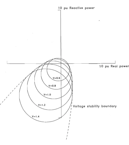
Figure 2.8 shows a series of load busbar voltage circles drawn on the
complex power plane; All of the circles fit into a parabolic region on
the plane. There are two possible busbar voltage solutions corresponding
to each complex load power within the parabola. Only one possible voltage
solution exists along the edge of the parabola and no solutions exist
outside the parabola.
Of the two possible voltage solutions that can be obtained within the
parabola, only the voltage with the larger magnitude is associated with a
stable operating point. The smaller voltage is associated with an
unstable operating point that will lead to a voltage collapse at the load
busbar. The rate of collapse is dependent on the type of load and may
occur over a period of several minutes (Venikov and Rozonov,1961 and
/ / /
/ /
/ /
10 pu Reactive power
I I I I
Figure 2.8 Voltage Circle Diagram
10 pu Real power
stability boundary
Each circle represents a locus of constant voltage
magnitude at the load busbar. All of the circles fit into a
parabolic envelope which represents the voltage stability
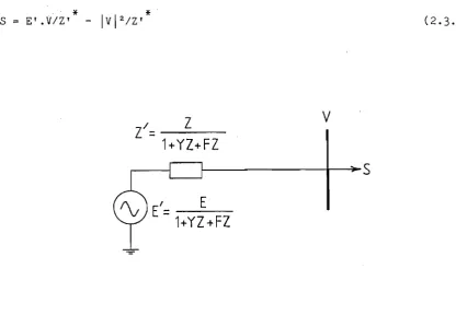
[image:36.562.64.504.88.581.2]Voltage Stability
The theoretical boundary of the stable voltage region is defined by
the parabolic envelope that contains the voltage circles. I t is
convenient to form a simple Th~venin equivalent of the circuit model to investigate the nature of the envelope. The Thevenin equivalent shown in
. figure 2.9 consists of a voltage source E' and a series impedance Z' where
E' EI (1 + 1. Z + F. Z) (2.3.2.2)
Z' ZI(1 + Y.Z + F.Z) (2.3.2.3)
The load busbar vol tage V and the load power S both retai n the same
significance in the Thevenin circuit.
The variables of the Thevenin circuit are related by the equation
S
v
~---r-~S
L--_...J
E'=
E
1+YZ+FZ
[image:37.562.64.481.342.630.2]The parabolic envelope is characterized by the existence of only one
solution for V corresponding to a given S in (2.3.2.4). This unique
solution can be found by first expressing the complex variables of
(2.3.2.4) in terms of their real and imaginary components. E' is used as
a real reference vector.
E' e + jO
S P + j q
V u + jv
Z' = r + jx
The solution for V in (2.3.2.4) in terms of u and v is then
u
v
e±l£e2
- 4[pr + qx + (qr-px)2/e 2J} 2
(qr-px)/e
(2.3.2.5)
(2.3.2.6)
The unique solution for V is identified by a zero valued argument in the
square root term of (2.3.2.5) . Hence V lies on the stability boundary if
u=e/2 •
The relationship between the stable and unstable solutions for V is
shown in the vector diagram of figure 2.10 • The original supply voltage
E is used as the reference vector and the theoretical stability boundary
is shown as a straight line bisecting the Thevenin voltage E'. As the
theoretical boundary is approached from the stable side the load voltage
fluctuations will become more pronounced until a total collapse occurs in
the unstable region.
A safety margin is provided by the practical stability boundary that
1 ies parallel to the theoretical boundary and intersects the Thevenin
voltage at 0.8E'. The factor of 0.8 1s a compromise between the need for
a reasonable safety margin and the need to allow for low but stable load
voltages. If a greater quality of voltage stability is required then the
factor of 0.8 should be increased.
If the shunt admittances are neglected then the Thevenin voltage E'
is identical to the original supply voltage E and the stability boundary
Unsta ble
r~glonTh~or~tical
stability boundary
/
/
for V
-4.-/
-+ Stabl~ r~glonfor
V
/
/
/
/
Practical stabi li ty boundary
/
~---r---+-~E
/
/
I
V
Figure 2.10 Relationship of Stability Boundary to Voltage Vectors
The theoretical voltage stability boundary bisects the
Thevenin equivalent voltage vector E' at a right angle. The
load voltage vector V should normally lie to the right of
the practical voltage stability boundary to allow for a
The theoretical and practical voltage stability boundaries are drawn
on the complex power plane by gradually shifting V along the appropriate
boundary in figure 2.10 and generating a sequence of S values from
"(2.3.2.4) . Both the theoretical and practical stability boundaries are
shown on the capability chart in figure 2.11 .
The maximum and minimum voltage limi ts are also represented on the
capability chart by arcs from the corresponding voltage circles that were
drawn in figure 2.8 .
Maximum Transmission Line Current
The maximum line current has been assumed to flow at one of the ends
of the line. The current entering the line from the supply end is 11 and the current leaving the line at the load end is 13•
The locus of the maximum current 11 can be obtained by using equations (2.3.1.2) to (2.3.1.4) to rewrite (2.3.1.1) in terms of 11 •
Th is yi elds
S (2.3.2.7)
where the complex constants A,B,C, and 0 are given by
*
*
*
* *
A E .(2.Y.Z+Y.Y.Z.Z +F.Z + F.Y.Z.Z )
* *
*
* * * *
*
B E.(1+Y.Z +Y .Z +Y.Y .Z.Z +F .Z +F .Y.Z.Z )
*
* *
*
C Z+Y .Z.Z +F .Z.Z
*
* *
*
*
* *
*
* *
D E.E .(2.Y+Y.Y.Z+2.Y.Y .Z +Y.Y.Y .Z.Z +F+F.Y.Z+F.Y .Z +F.Y.Y .Z.Z )
Equation (2.3.2.7) describes an elliptical locus as the magnitude of 11
Minimum
2 pu Reactive power
Maximum line current
\ I I I Practical voltage stability limit I I Theoretical voltage stability limit I
Figure 2.11 Capability Chart of Transmission Line
The shaded area denotes the range of real and reactive
power that may be supplied to the load. This area is bounded
by loci that represent the critical operating limits of the
At the load end of the line the locus of 13 can be found in a similar
fashion by rewriting (2.3.1.1) in terms of 13 , This yields
s
(2.3.2.8)where the complex constants A,B,C, and D are given by
* *
A E .F • Z 11 + Y.Z/2
*
E. ( 1 + 1. Z + F.Z)
B
11 + Y.Z/2
*.
C Z. ( 1 + 1. Z + F.Z)11 + Y.zI2 IE 12.F
*
D
11 + Y.zI2
Equation (2.3.2.8) also describes an elliptical locus as the magnitude
of 13 is held constant and the phase angle is varied through 360 degrees.
If the shunt admittance F is zero then this locus becomes circular.
The two loci of maximum current are indistinguishable on the
capabili ty chart of figure 2.11 • The ellipses become more distinct as
2.3.3 Capability Chart on the Admittance Plane.
If the load is a soft admittance load rather than a stiff constant
power load then it is more appropriate to draw the capability chart on
the complex admittance plane instead of the complex power plane. The
chart on the admittance plane is shown in figure 2.12 .
The maximum and minimum load voltage limits and the maximum line
current 1 imit are shown on the admittance chart. A vol tage stabU i ty
limit is not shown because the voltage collapse phenomenon does not exist
for pure admittance loads.
2 pu Susceptance
aximum voltage
voltage
Maximum line current
Figure 2.12 Capability Chart of Transmission line on the
If the complex power S is replaced by a complex load admittance G
then G is given by
G (2.3.3.1 )
This equation is used in place of the complex power equation (2.3.1.1)
to formulate the equations describing the constraint loci on the complex
admittance plane.
Voltage Limits
The loci corresponding to the maximum and minimum load voltage are
obtained by combining (2.3.1.2), (2.3.1.4) and (2.3.3.1) to yield
G E 1 ( V • Z) - ( 11 Z + F + Y) (2.3.3.2)
If the magnitude of V is held constant at the maximum or minimum value
and the phase angle of V is varied through 360 degrees then (2.3.3.2)
describes a circle on the complex admittance plane. The radius of the
circle is IE/(VZ)I and the centre is at -(1/Z+F+Y) .
Two arcs from the voltage circles are drawn on the admittance chart
in figure 2.12. The voltage circles are concentric and their common
centre represents the shunt admittance that would produce a resonance
between the series impedance Z and the shunt admittances Y, F, and G at
the load busbar.
Line Current Limit
The locus of maximum current entering the line from the supply bus bar
is obtained by using (2.3.1.2) to (2.3.1.4) to rewrite (2.3.3.1) in
terms of II'
If the magnitude of II is held at its maximum value and the phase angle
of II is rotated through 360 degrees then (2.3.3.3) describes an ellipse
on the admittance plane.
The locus of maximum current leaving the line at the load busbar is
also elliptical and is found by rewriting (2.3.3.1) in terms of 13 to
give
G 13.(1 + Y.Z) ._ F
E - 13'Z
(2.3.3.4)
The two elliptical loci of maximum current flowing through the ends
of the line are indistinguishable on the admittance capability chart. As
with the power capability chart the loci gradually become separated if
the line shunt admittances of Yare greatly increased in value.
2.3.4 Summary of Transmission Line Capability Charts
Two capability charts have been constructed to describe the
performance of a transmission line. One chart is drawn on the complex
power plane and the other is drawn on the complex admittance plane.
The operating limits represented on the complex power chart are the
minimum and m.aximum voltage at the load busbar, the voltage stability
boundary, and the maximum current flowing at either end of the line.
These limits are also represented on the complex admittance chart
apart from the voltage stability boundary which is not applicable.
Power system operators tend to regard loads from the complex power
viewpoint rather than the complex admittance viewpoint. This tendency
reduces the importance of the admittance capability chart. The predominance
of the complex power viewpoint has also influenced the rest of the work
2. ~ CONCLUSION
This chapter has described the capability charts for two simple power
systems. First the chart for a salient pole generator is constructed by
using the method described by Walker (1953). The round rotor generator is
regarded as a special case of the salient pole machines.
The chapter then describes the capability chart for a transmission
line. The traditional voltage circle diagrams are used to construct the
loci that represent maximum and minimum voltage limits. The equations of
other loci are then derived to represent the maximum line current and
voltage stability limits.
A capability chart for the transmission line is also constructed on
the complex admittance plane which is more appropriate for admittance
loads. The admittance chart is not considered in the rest of this thesis
because of the prevalent tendency to regard loads in complex power terms.
The equations of the loci for these simple systems are derived by
algebraic and geometrical manipulation of the basic operating equations
and vector diagrams. This technique is restricted to small systems
because the algebraic manipulation rapidly becomes too unwieldy as the
Chapter 3
A Chart for an HVDC Link
3.1 INTRODUCTION
The development of a capability chart to describe the steady state
performance of an HVDC link is particularly attractive because of the
increasing use of HVDC links in power systems. Kimbark (1971) developed
charts to describe the operation of individual static converters, but a
capability chart for a complete HVDC link has not been considered before.
The work described in this chapter has been accepted for publication by
the lEE (de Silva, Arnold, and Arrillaga, 1987).
The HVDC link capability chart is constructed by using a similar
techni que to that used for simple systems, such as the synchronous
generator and transmission line described in chapter 2. The basic
operating equations that describe the behaviour of the HVDC link are
manipulated into a suitable form for drawing loci on the complex power
plane.
A simplified model of the New Zealand Benmore-Haywards HVDC link has
been chosen to demonstrate the construction of the capability chart. The
technique used is also applicable to any other two terminal HVDC link.
3.2 CIRCUIT MODEL OF THE HVDC LINK
The New Zealand HVDC link can transfer 600 MW between the North and
South Islands of New Zealand. The southern terminal of the link is at
Benmore power station and the northern terminal is at Haywards. 600 km of
overhead transmission line and ~O km of undersea cable connect the two
terminals.
A circuit diagram of the HVDC link is shown in figure 3.1 • The locus
equations described in chapter 2 for single generators and transmission
lines were not simple to derive. This indicates that considerable
equations for the actual HVDC scheme which includes several transformers,
generators, and AC/DC converters. Therefore the simplified circuit model
shown in figure 3.2 has been chosen instead for the development of the
capability chart.
At the Benmore converter terminal the six 90 MW hydro-electric
generators are modelled by a single equivalent 5~0 MW generator feeding a single 16 kV busbar. The voltage level of the busbar is regulated by the
generator AVR. The equivalent generator can also operate as a synchronous
compensator to deliver up to 32~ MVAR or consume a maximum of 378 MVAR.
The two three-windi ng transformers that interconnect the 16 kV
busbars and the South Island 220 kV system are modelled by a single, two
winding, ~OO MVA interconnecting transformer, having a
3.3
%
reactance. This reactance is derived from a power base of 100 MVA that has beenchosen for the entire AC/DC system.
The two banks of harmonic filters that are attached to the tertiary
windings of the three-winding transformers are modelled as a single bank
of filters attached to the 16 kV busbar. The filters absorb th~ harmonic
currents from the converter and also supply 100 MVAR of reactive power.
The behaviour of these filters is considered to be ideal so that the
voltage waveform on the 16 kV busbar is assumed to be sinusoidal. This
assumption is adequate for a steady state, fundamental frequency analysis
of the HVDC link.
The converter terminal at Benmore consists of two 250 kV DC poles.
Each pole consists of two six pulse bridges in series. The mercury arc
valves in the bridges are rated to carry a continuous DC current of 1.2
kA . A 30 degree phase difference between the converter transformers
allows an overall twelve pulse operation for each pole.
The four bridges operate under identical control so the bridges and
converter transformers can be modelled by a single equivalent twelve
pulse bridge and transformer (Arrillaga et al., 1983). The equivalent
bridge is rated to carry 1.2 kA DC current. The equivalent lossless
converter transformer is rated at 750 MVA and has a reactance of 2%
Since it has been assumed that the converter transformer is fed from a
sinusoidal voltage source, the transformer reactance can also be regarded
An overhead transmiss ion 1 ine and an undersea cable transmit the
power from the Benmore converter to the Haywards converter. The large
smoothing reactors at each end of the line are assumed to maintain a
constant DC current. The total resistance of the converters, smoothing
reactors, transmission line, and cable is 25.56
o.
The Haywards converter terminal also consists of four six pulse
bridges in series. The three winding converter transformers connect the
bridges to a 110 kV busbar as well as to four synchronous compensators.
This arrangement is modelled by a single equivalent bridge, and a two
winding converter transformer. The equivalent bridge and transformer have
the same parameters as the equivalent Benmore converter.
In the model, the synchronous compensators are connected directly to
the 110 kV busbar instead of a tertiary transformer winding. This
particular simplification introduces the greatest error in the modelling
of the. Benmore-Haywards scheme, but also results in a closer
correspondence to other HVDC schemes that use two winding converter
transformers (Vancouver Island, Pacific Intertie, Skagerrak, Square
Butte, CU, Nelson River Bipole II, Inga-Shaba, and Gotland II).
The voltage level of the 110 kV busbar is maintained by the AVR on
the equivalent synchronous compensator which can provide up to 260 MVAR
of reactive power. This is supplemented by 110 MVAR from the harmonic
filters which are assumed to maintain a sinusoidal voltage on the busbar.
The 110 kV busbar feeds the North Island AC network.
Similarly to the capability chart of a synchronous generator, which
represents the complex power available from the generator terminals, the
most useful information to be derived from the HVDC link capability chart
is the complex power available to the Haywards 110 kV busbar from the
220kV
South
Island
Line Cable 110 kV
1---11----11 ~r·
North Island
l---+---ll ~I'
BENMORE HAY'w'AROS
South
Island
540MW
220 kV
V
dc
[ ) 260 MVAR
Vac
~ 7
>-
>North
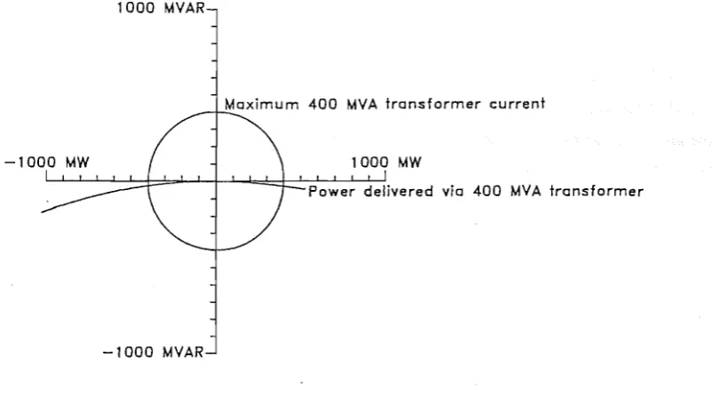
4-00 MVA
P
+jQ
Island
'1r--rrrY
100 M VAR Fi l
ters
BENMORE
Figure 3.2 Simplified Model Of New Zealand HVDC Scheme The capability chart of the HVDC link portrays the real and reactive power (P+jQ) that can be supplied from the Haywards converter transformer to the Haywards 110 kV busbar.
~II
110 MVAR
HAYWARDS
w
3.3 OPERATING CONSTRAINTS OF THE HVDC LINK
Each operating constraint of the HVDC link must be represented as a
locus on the capability chart.
Converter Transformer Current
The heat dissipation capability of each 750 MVA converter transformer
determines the maximum RMS current that may flow through the transformer
windings. This current consists of a fundamental frequency component as
well as several harmonic frequency components. All of these components
must be considered even though only the fundamental current contributes
to the useful power available.
Converter Valve Current
The DC line current flows through the converter valves, smoothing
reactors, transmission line, and cable. Of these four components, the
converter valves possess the smallest current rating of 1.2 kA, and they
therefore determine the maximum DC current that may flow in the link.
The converter valves also require a minimum holding current of 0.1
kA. This is the DC current necessa~y to sustain valve conduction whilst each valve is nominally on.
Harmonic Filter Current
The DC line current is also related to the harmonic currents flowing
in the filter banks. If commutation effects are neglected then the
harmonic current levels can be assumed to be directly proportional to the
DC current. This is a safe assumption because the inclusion of
commutating effects tends to reduce the calculated harmonic current
levels (Arrillaga, 1983).
The f il ters are designed to cope with the harmonic currents
associated with the maximum expected DC current, as well as the
maximum converter valve current locus will also ensure a safe level of
harmonic filter current.
DC Voltage Rating
The DC voltage of the transmission line and cable has a reasonably
smooth waveform during steady state operation. The maximum continuous DC
voltage that may be borne is 525 kV. This is determined by the continuous
voltage ratings of the transmission line insulators, surge arrestors, and
cable insulation. Each of these components will also tolerate a much
higher transient overvoltage, but this is not represented on the steady
state capability chart.
Converter Control Angles
A minimum limit is set on both converter control angles. During