The Atmospheric Gravity Wave Transfer Function above Scott Base

(1)

Department of Physics and Astronomy, University of Canterbury,

Private Bag 4800, Christchurch, New Zealand

The Atmospheric Gravity Wave

Transfer Function above Scott Base

A Thesis Submitted in Partial Fulfilment

of the Requirements for a

Masters Degree in Physics

at the University of Canterbury

by

Andr´e Geldenhuis

University of Canterbury, 2008

Supervisors: Dr A. McDonald

(2)

(3)

List of Figures

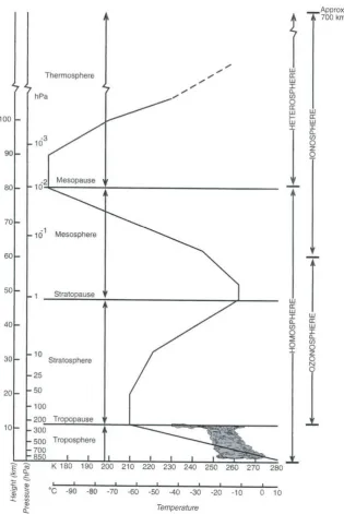
2.1 Vertical structure of the atmosphere. (Sturman and Tapper, 2006) . . . 8 2.2 Zonal and meridional winds during the December solstice using HWM 93

model data. The zonal winds divides quite naturally into 3 layers: The lower atmosphere from approximately 0-20km, the middle atmosphere (encompass-ing both the stratosphere and mesosphere) from roughly 20-80km, and the upper atmosphere above 80km. . . 9 2.3 Zonal winds during the June solstice. Note that the stratospheric summer jet

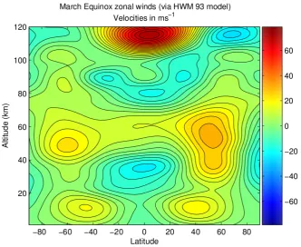
is in the westward direction. . . 9 2.4 Zonal wind velocities during the March equinox. In this configuration, the

sun heats the equatorial stratosphere more than the pole, causing the middle atmosphere jets to both blow east. . . 10 2.5 Zonal and meridional winds at Scott Base via the HWM 93 model. . . 11 3.1 Topographically generated gravity waves. Adapted fromGerbier and Berenger

(1961). . . 14 3.2 An image from the NOAA-14 satellite on the 4th_{of October 1999. Taken from}

Dean (2002) . . . 15 3.3 Spaced array techniques (Hocking, 1997). Radar is backscattered producing

a Fresnel diffraction spot on the ground. The equilateral triangle of receiv-ing antennas allows the velocity of the diffraction spot to be measured, this corresponds to the movement of the scattering layer. . . 17 3.4 Amplitude of a Fresnel diffraction spot moving over three antennas. From

Briggs (1984). . . 18 3.5 Simple model of breaking wave breaking from (Andrews et al., 1987). . . 25 4.1 The wave periods present in the radar wind data in 2007. The dashed line is

the 99% significance level. . . 28 4.2 Example of radar gravity wave energy quality control . . . 29 4.3 Averaging the gravity wave kinetic energy for each height bin and year. . . . 30 4.4 An early analysis of the variations in gravity wave energy between the years

(6)

4.5 Gravity wave climatology derived from the Scott Base MF-radar over 2005 to early 2008. Derived from variances of the wind residuals after removing tidal components. Smoothed with a 10% sliding window. . . 32 4.6 Gravity Wave climatology 1985-2003, prior to the upgrade of the data

ac-quisition system of the Scott Base MF-radar. Smoothed with a 10% sliding window. . . 32 4.7 Climatology of monthly mean wind variances between 1997 and 2005 at

Rothera, from Hibbins et al. (2007). These wind variances are taken to be associated with gravity wave activity. . . 33 4.8 Climatology of zonal and meridional wind variances after removal of tidal

components at Davis (top panel) and Syowa (bottom panel). Adapted from

Dowdy et al.(2007). . . 34 4.9 Variability of gravity wave kinetic energy between years and before and after

data acquisition upgrade. . . 34 5.1 McMurdo radiosonde sampling altitude statistics between 1 and 8km. Each

balloon flight between 2000 and the start of 2007 is displayed. The aver-age difference in altitude between measurements is displayed, as well as the maximum and minimum difference for each flight. . . 37 5.2 Another way of examining the radiosonde’s data sampling is to calculate the

least squares linear slope of differences in height vs. sample number. . . 38 5.3 The total mean gravity wave kinetic energy between 1−8kmand 9−13kmat

200m vertical resolution. All means and standard deviations is smoothed with a 15 day running mean. As the data in the period after September 2004 was of a higher quality, the mean kinetic energy per unit mass was re-calculated after this time binned at 40m rather than 200m. . . 40 5.4 The mean gravity wave kinetic energy per unit mass in the troposphere in

2000-2007. In 2000-2004 the data quality was lower (detailed in Figure 5.1 and 5.2). The mean and standard deviation are smoothed with a 15 day running mean . . . 40 5.5 Potential energy associated with gravity waves between 9 and 13km. As the

data in the period after September 2004 was of a higher quality, the mean kinetic energy per unit mass was re-calculated after this time binned at 40m

rather than 200m. . . 41 5.6 Mean gravity wave propagation direction between 1−8kmand 2000-2007 with

(7)

List of Figures 3 6.1 Fictional blocking circle in the lowest height bin due to a meridional wind

blowing directly toward the north (northward) with no zonal component. The blue circle represents the range of phase speeds and wave directions that will be unable to pass through this altitude. The red lines represent gravity waves with certain phase speeds and horizontal directions. The wave inside the blocking circle will be unable to propagate higher while the other wave has a sufficient phase speed to pass through the potential critical level. . . 45 6.2 Composite blocking circles “looking down” from the third height bin on a

certain day or time period. As successively higher altitudes are examined the meridional wind component grow weaker while a eastward wind strengthens. This can be seen by the coordinates of the successive blocking circles (U, V) It can be seen that the gravity wave which was able to pass through the first and second bins reaches a critical level by the third bin and is stopped. . . . 45 6.3 By restricting the Monte Carlo random numbers to the eastward quadrant, the

blocking of waves propagating in the eastward direction could be studied. By repeating this for the remaining cardinal directions and a range of maximum phase velocities it is possible to identify a relatively comprehensive overview of wave blocking. . . 47 6.4 A test of the Monte Carlo method using equation 6.3 and a background wind

of 15ms−1 _{toward the east (the right hand side of the diagram). The points}

are random phase speeds with a maximum phase velocity of ±20ms−1 _and

a random propagation direction. The red points are considered blocked by equation 6.3. The fraction of waves blocked in this example is 0.14 or 14% . 48 6.5 Testing for the optimum number of points for the Monte Carlo wave blocking

calculation. The blue points represents how close each run was to an ideal case. The ideal case was taken to be the result of a ten million point run. Each run used a different number of randomly generated points, repeated 100 times to obtain a meaningful spread of points. The red line and green line show one and two standard deviations in difference respectively. . . 48 6.6 The blocking of small phase velocity waves as the wind vector rotates between

two height bins. The red line indicates the wind vector in the first altitude bin while the green indicates the wind vector in the second bin. The shaded area indicates the degree to which low phase velocity waves are blocked. . . 50 6.7 Blocking of small phase velocity gravity waves between 4 altitude bins. Note

that between the 3rd and 4th height bin the wind vector starts to move back toward the direction of wind in the second height bin. These reversals need to be taken into account . . . 50 6.8 Filtering scheme for gravity waves with a phase speed between 0 and 5ms−1_.

The lower panels show the blocking field separated into NSEW filtering com-ponents. . . 53 6.9 Filtering scheme for gravity waves with a phase speed between 0 and 20ms−1_.

(8)

6.10 Filtering scheme for gravity waves with a phase speed between 0 and 40ms−1_.The

lower panels show the blocking field separated into NSEW filtering components. 55 6.11 Summer and winter gravity wave blocking circles at Davis (69◦S,78◦E) and

Syowa (69◦,40◦E) stations. Calculated from the ground up to approximately 56km. FromDowdy et al. 2007 (Modified to show Antarctic locations only) . 56 6.12 Filtering scheme for phase speeds between 0-1ms−1_{. This should be}

represen-tative of mountain wave filtering. . . 56 6.13 Filtering scheme based on wind rotations. The wind field is checked for

rota-tions of more than 180 degrees from the ground up. Where this has occurred mountain waves are considered completely blocked. Lesser degrees of rotation are shown as a fraction of 180 degrees rotation. . . 57 6.14 NCEP/NCAR reanalysis based gravity wave blocking between 0 and 20ms−1 ₅₇

6.15 Hybrid filtering scheme for phase speeds between 0-5ms−1 _{. . . .} ₅₈

6.16 Hybrid filtering scheme for phase speeds between 0-20ms−1 . . . 59 7.1 Log of residual fits of the tropopause source function (9-13km) and model

wave passing field (with suitable exponential growth term) to the observed gravity wave field at 75-96km . . . 63 7.2 Log of residual fits of the tropopause source function (9-13km) and the radar

(9)

Chapter 1 Introduction

“Despite the recognised importance of gravity wave processes to problems of general circula-tion, relatively little is known about their relative strengths and frequencies of occurrence” (Nastrom and Fritts, 1992). While progress has been made in the 15 years since this quote, the difficulties in observing these atmospheric features has not reduced its relevance.

1.1 Motivation

Gravity waves have been theorised to exist since Lord Rayleigh first considered stability effects in the atmosphere. Indeed, early work with meteor radar and radiosondes made mea-surements of relatively rapid perturbations to the background flow. Hines (1960) clearly notes that these winds could be due to internal gravity waves propagating from the tro-posphere and growing exponentially with height. In the early 1980’s, several papers were published suggesting that gravity waves could play a significant role in mesospheric dynamics through the transport of momentum from the lower atmosphere (see Lindzen, 1981; Holton, 1982).

The understanding of the particular importance of gravity waves came at a fortuitous time, as recent developments by University of Canterbury researchers at the Birdlings Flat site had lead to the use of MF-radar to measure winds through the observation of radar backscatter from partial ionisation in the D-region of the atmosphere (Fraser, 1984a). While MF-radar had been used to determine mesospheric winds prior to this, the use of radar backscatter allowed measurements to be taken of winds at lower altitudes than previous full reflection methods allowed. At lower altitudes the collision frequency between the ionised and neutral gas is sufficiently high that the ionised gas velocities can be assumed to be representative of the neutral gas velocity.

While the field of gravity wave study has matured since its early days, there are still a great many areas in which more research is needed. During a gravity wave conference in 2006, several areas where an improvement in understanding of gravity waves was needed were highlighted. One of these areas was that of gravity wave sources and propagation (Geller et al., 2006). For this reason, this thesis aims to provide a greater understanding of gravity wave sources and propagation above Scott Base, Antarctica, and their relative importance

(10)

on the observed mesospheric gravity wave field.

1.2 Structure

The following two chapters of this thesis give a general overview of atmospheric dynamics and structure, and gravity wave theory.

Chapter 4 uses data from the Scott Base MF-radar, run by the University of Canterbury. Recently, this radar was upgraded to improve its ability to resolve gravity waves above the background noise level (Baumgaertner et al., 2006). In order to resolve gravity waves, atmospheric tides and larger scale perturbations are removed from the wind data. The variance of these perturbations is taken to be due to gravity waves. Using this method, a gravity wave climatology is produced which spans the years after the radar upgrade, from 2005 to early 2008.

Chapter 5 details the use of radiosondes launched from McMurdo (which is very close to Scott Base) to determine a gravity wave source function. This source function takes the form of a climatology of kinetic energy due to gravity wave perturbations. Unfortunately, there was a significant change in the McMurdo radiosonde program in late 2004, which, combined with the public availability of the McMurdo radiosonde data set ending in 2007, left little more that two years of good data. To discern the effect of using such a small data set, a gravity wave climatology for the years before the program change was also calculated covering 2000 - 2004. Comparing the mean kinetic energy before and after the change, it was determined that the post-upgrade data was sufficiently representative to be used as a gravity wave source function.

Chapter 6 uses wind data from the Horizontal Winds Model 93 (HWM 93) to develop a gravity wave filtering function model based on critical level filtering and blocking circles. This atmospheric transfer function is calculated for several ranges of potential gravity wave phase speeds and propagation directions. The transfer function indicates the degree to which gravity waves with certain properties (such as phase speed and propagation direction) are blocked as they move up through the atmosphere.

(11)

Chapter 2 Atmospheric Dynamics

2.1 Structure

At the broadest scale, the structure of the Earth’s atmosphere varies horizontally from the equator to the poles. These variations are due to different energy deposition rates and the Coriolis Effect.

The vertical variations are similar enough over the globe that the changes in temperature gradient as a function of height are used to identify different regions of the atmosphere. Based on these changes in temperature gradient (or lapse rate), the atmosphere can be divided into several different altitude regions, shown in Figure 2.1. The first is the troposphere, starting from the ground and extending to approximately 10 -15km. This region is warmed primarily by heat radiating from the ground and cools increasingly with altitude as clouds and water vapour radiate heat into space (Andrews et al., 1987). The cooling trend in the troposphere makes it almost dynamically unstable; moist rising air masses can remain warmer than the surrounding air due to water droplets condensing and releasing their latent heat into them. Since the air mass is warmer than its surroundings it can continue to rise, causing this region to be well mixed.

The variation in solar heating from the equator to the poles results in horizontal tem-perature gradients. This gradient forces air masses away from the equator. However, as the equator is further from the planet’s axis of rotation, these air masses posses greater angular momentum than they would at higher latitudes. As such, conservation of angular momen-tum dictates that as air masses move eastward (prograde), they also try to move toward the poles. This results in the eastward tropospheric jets used by airlines to decrease travel times on eastward-bound flights. Because the tropospheric equator is always warmer than the poles, these jets move to the east regardless of the season.

At greater altitudes the low temperatures reduce the amount of water vapour that the air can contain. Above the troposphere the atmosphere is very dry, and warms increasingly with altitude. The change from cool to warm air and the very low humidity are signatures of the stratosphere. This warming is due to the rapid rise in ozone above the tropopause. Ozone strongly absorbs UV light, depositing energy into the stratosphere. The amount of ozone peaks in the lower stratosphere. However, temperature continues to rise with altitude

(12)

[image:12.595.119.435.162.634.2]

(13)

2.1. Structure 9

Figure 2.2: Zonal and meridional winds during the December solstice using HWM 93 model data. The zonal winds divides quite naturally into 3 layers: The lower atmosphere from approximately 0-20km, the middle atmosphere (encompassing both the stratosphere and mesosphere) from roughly 20-80km, and the upper atmosphere above 80km.

(14)

Figure 2.4: Zonal wind velocities during the March equinox. In this configuration, the sun heats the equatorial stratosphere more than the pole, causing the middle atmosphere jets to both blow east.

due to decreasing atmospheric density (requiring less energy to heat).

This heating by ozone-absorbing UV light is the primary warming mechanism in the stratosphere. This leads to some interesting differences to the tropospheric region. Since the summer pole receives far more irradiance than the equator, the high latitude summer strato-sphere is warmer than the equatorial stratostrato-sphere because of radiative heating. This leads to a reversal of the summer stratospheric jet. Due to conservation of angular momentum, as air masses attempt to move toward the equator they will appear to to be forced toward the west, resulting in a westward (retrograde) summer jet. The equatorial stratosphere is still warmer than the winter stratosphere at this height, hence the winter jet is eastward, similar to the tropospheric jets (see Figure 2.4).

The temperature trend in the stratosphere makes it very stable. Any vertically displaced parcels of air will attempt to return to its equilibrium position, oscillating until damped. This oscillation makes the stratosphere an excellent medium for the propagation of gravity waves, which will be discussed in the next chapter.

[image:14.595.111.444.57.329.2]

(15)

2.2. Atmospheric waves 11

Figure 2.5: Zonal and meridional winds at Scott Base via the HWM 93 model. EM field. Another interesting feature of this region is that at high latitudes the winter mesosphere is warmer than in summer. This has been attributed to the action of breaking gravity waves (Geller, 1983).

The final region considered in this thesis is the lower thermosphere. This region begins where the temperature starts to increase above the mesopause at around 85km. The temper-ature increase in this region is due to the absorption of high energy UV radiation from the sun (Kelley and Heelis, 1989). As the electron density due to ionisation grows quickly in this region, this thesis will confine itself to altitudes of 96km and below where electromagnetic effects on the plasma in this region can be considered to have an insignificant effect on the motion of the neutral component of the atmosphere.

2.2 Atmospheric waves

Atmospheric waves play a significant role in the dynamics of the atmosphere. They are par-ticularly important in coupling different regions together. The action of large scale planetary waves is the mechanism by which tropical convection can influence extra tropical dynamics (Salby, 1996). Indeed it shall be shown in the following chapter that short period atmo-spheric waves (internal gravity waves) can provide coupling between the troposphere and the mesosphere, driving the dynamics in the latter region.

The largest-scale atmospheric waves are the planetary waves and Rossby waves which have diverse effects on the atmosphere. These waves can transport heat and momentum to high altitudes which is released by wave breaking. For instance, it has been demonstrated that the breaking of these large scale waves can decelerate the polar vortex leading to the vortex breakup up earlier in the season (Holton and Alexander, 2000).

Another type of large scale wave are atmospheric tidal waves. These waves are generated via several mechanisms, the most significant is solar heating (Chapman and Lindzen, 1970). The tidal modes considered in this thesis are harmonics of the solar driven diurnal tide.

(16)

(17)

Chapter 3 Gravity Waves and Observational

Techniques

“Despite the recognised importance of gravity wave processes to problems of general circula-tion, relatively little is known about their relative strengths and frequencies of occurrence” (Nastrom and Fritts, 1992).

3.1 Gravity waves

Waves with the restoring forces of gravity and buoyancy are known as gravity waves. These waves are present through much of the atmosphere with periods between the Brunt-Väisälä period and inertial period.1 _{There are many mechanisms by which these waves can form;}

however, the gravity waves above Scott Base (which are examined in this study) are likely to be predominantly formed by winds passing over the Trans-Antarctic mountain range (Baumgaertner and McDonald, 2007). As the air passes over the ranges it is displaced from its equilibrium position and oscillates around this height position as it moves down-wind of the mountain, creating a wave. The air column above is also displaced, allowing the gravity wave to propagate almost vertically well into the thermosphere.

These waves provide much of the coupling between the lower and upper atmosphere by transporting energy to higher altitudes2_{. This is particularly important in the Antarctic}

MLT, as this is the region of the atmosphere farthest from radiative equilibrium (Gill, 1982). For example, the winter temperature in the MLT above the polar regions is generally higher than that in summer. While at first glance this observation may appear unexpected, it has been shown to be related to the forcing associated with gravity waves. The energy transported by gravity waves has also been shown to control the strong mesospheric winds and play a significant role in closing the stratospheric jets(Lindzen, 1981; Holton, 1982).

The stratospheric jets define the polar vortex, the strength of which determines the degree of mixing between the Antarctic and the mid-latitude stratosphere (Krutzmann et al., 2008). The degree of mixing therefore plays an important role in ozone dynamics. As such,

1_{infinite at equator to 12 hours at poles(Fritts and Alexander}_{, 2003)} 2_(See_Hamilton _{(1999) for an overview of the discovery of this phenomena)}

(18)

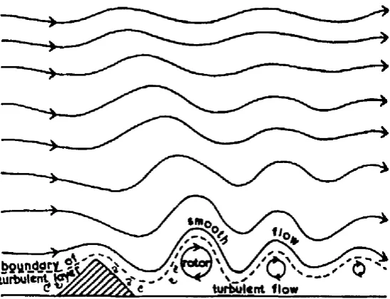
Figure 3.1: Topographically generated gravity waves. Adapted from Gerbier and Berenger

(1961).

the study of internal gravity waves in the Antarctic atmosphere is important to further our understanding of these phenomena.

3.1.1 Sources of gravity waves

There are a variety of gravity wave sources in the atmosphere, while some of these sources are not significant in the Antarctic, the main sources shall be briefly detailed below.

Perhaps the most easily understood source of gravity waves is topographic generation. As wind blows over a mountain range packets or parcels of stable air are vertically displaced. As these parcels move downwind from the mountain range, they seek to return to their equilibrium position due to the effect of gravity as they are denser than the surrounding at-mosphere. However they tend to overshoot this position at which point the force of buoyancy acts to reverse their motion as they are now less dense than the surrounding medium. This process is illustrated in Figure 3.1. A notable property of mountain waves is that their phase speed is locked to the topography below. This will be shown to be particularly important when wave breaking and wave drag are considered.

Another source of gravity waves is geostrophic adjustment around jets. Large scale move-ments of the atmosphere tend to remain in balance with all the forces that would act on them, as this is the lowest energy state. However, as the atmosphere is a dynamic environ-ment with many competing effects, these large scale motions are often not in balance.This can be the case around jets in the atmosphere as their large scale enables them to alter the geostrophic balance of the atmosphere. (de la Torre and Alexander, 2005). A return to the lowest energy state, in this case termed geostrophic adjustment, requires the radiation of energy. In the atmosphere this energy is radiated away in the form of gravity waves.

[image:18.595.137.411.63.273.2]

(19)

3.2. Observation methods 15

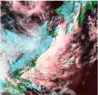
Figure 3.2: An image from the NOAA-14 satellite on the 4th_{of October 1999. Taken from}

Dean (2002)

waves away – though the actual mechanism is non-linear (Buhler and McIntyre, 1999). Both wind shear and geostrophic adjustment radiate gravity waves with phase speeds similar to the wind speed with which they are associated (Sutherland and Peltier, 1995).

Strong convection is another mechanism which can produce gravity waves (Fritts and Alexander, 2003). However, the Antarctic is too cold for any significant convective activity so this gravity wave source shall not be considered in this thesis.

3.2 Observation methods

Gravity waves can be observed in a variety of ways. At the simplest level, gravity waves can occasionally be seen as lee clouds when wind flows over a mountain range. There are a variety of more sophisticated optical observational methods, ranging from air-glow images taken at night, to satellite images of clouds associated with gravity waves (see Figure 3.2). Satellite-based instruments are also able to obtain temperature profiles, often by limb sounding or radio occultation techniques. These temperature profiles can be used to determine larger-scale gravity wave activity.

[image:19.595.155.478.61.374.2]

(20)

verification of satellite results.

The two techniques that this thesis uses to acquire gravity wave data are MF-radar and radiosondes. These two techniques are presented in more detail below.

3.2.1 Scott Base MF-radar

The Scott Base MF-radar measures horizontal winds in the mesosphere and lower thermo-sphere (MLT). The radar transmits pulses which are partially reflected from the D-region of the ionosphere, and produce diffraction patterns which can be observed at the ground. The radar measures wind speeds by analysing the movement of these diffraction patterns using a set of spaced receiving antennas. In the following chapter, the atmospheric tidal signals are removed from this wind data in order to identify the wind perturbations due to gravity waves alone, albeit with some degree of noise.

The Scott Base MF-radar consists of the transmitter at Scott Base, Antarctica (77◦510S, 166◦450E) and a spaced receiving array at Arrival Heights 3.3km away (Fraser, 1984a). The radar operates at a frequency of 2.9Mhz, with a peak power of 100kW. The transmitter currently has a pulse repetition frequency of 30Hz, although it has been lower in the past (Baumgaertner et al., 2006; Fraser, 1984b).

The transmitting antenna and three receiving antennas are all deltas (triangular anten-nas). Because delta antennas have an almost isotropic radiation pattern they are not optimal for observing the atmosphere above the radar.3 _{However, deltas have been shown to be more}

resistant to wind and ice stress problems (Fraser, 1984b), which is particularly important in the Antarctic where antenna maintenance can be a daunting task even during the relatively mild summer months.

The transmitting antenna is a single, open-wire delta located very close to the Transmitter Hut which is short walk from the Hatherton Laboratory. The receivers are located at the new Arrival Heights Laboratory with the antennas spaced near by. The three antennas which comprise the receiving array are arranged in an equilateral triangle with spacing between their phase centres approximately 125m apart. Snow flakes carry a static charge which manifests as receiver noise and therefore the receiving antennas are insulated to prevent this.

The signal of interest that is returned from the atmosphere is a partial reflection of the radar waves caused by variations in the radio refractive index of the atmosphere. These variations are due to electron density increasing with altitude and horizontal variations (Manson and Meek, 1984). The horizontal variations are of the correct scale for Fresnel diffraction of the backscatterered radar wave to occur, which produces a diffraction spot on the ground.

Assuming that the horizontal variation in electron density moves with the background wind, the movement of the diffraction pattern at the surface will be directly related to the winds at the reflection altitude. However, since electrons are required in order to produce the diffraction pattern, the assumption that the variations are moving with the background

3_{If the antenna pattern is directed upward, this has the dual effect of increasing the system’s gain as well}

(21)

3.2. Observation methods 17

Figure 3.3: Spaced array techniques (Hocking, 1997). Radar is backscattered producing a Fresnel diffraction spot on the ground. The equilateral triangle of receiving antennas allows the velocity of the diffraction spot to be measured, this corresponds to the movement of the scattering layer.

wind is only valid when electrons are colliding frequently with neutral atoms. At altitudes higher than 95 to 100km, the collision frequency is low enough that the electrons become increasingly affected by geomagnetic effects and this assumption is no longer valid (Fraser, 1984b). Therefore, the radar winds were taken from an altitude range of 75 to 96km.

To determine the horizontal wind speed, the movement of the diffraction spot is observed by the three receiving antennas. Each antenna detects a portion of the diffraction spot. There are two methods by which the antenna and associated receiver do this: the least complicated method is to use a simple amplitude receiver, which measures the contours simply as changes in received signal strength. A more sophisticated method uses phase-sensitive receivers to obtain more information about the returned signal. For simplicity, only the amplitude changes method will be described. Note that most modern MF-radars (such as the radar at Scott Base) use these phase-sensitive receivers although the basic concepts are applicable to both.

As a diffraction spot moves over the receivers (see Figure 3.3) it produces changes in the amplitude of the received signal. If there were many more than three receiving antennas, it would be simple to track the motion of the diffraction spot since it could effectively be imaged. However, the motion of the diffraction spot can still be determined even with only three antennas.

[image:21.595.135.499.68.296.2]

(22)

Figure 3.4: Amplitude of a Fresnel diffraction spot moving over three antennas. FromBriggs

(1984).

at different receiving points can then be compared using a technique called Full Correlation Analysis (FCA), which is clearly detailed in Briggs (1984).

Currently the Scott Base MF-radar takes measurements for one minute while the FCA algorithm is run on the previous minutes data. The FCA algorithm is used to calculate horizontal winds from 60km to more than 100km. As most of the mechanisms responsible for ionisation in the D-region of the ionosphere are due to sunlight, the D-region effectively disappears at night (Nicolet and Aikin, 1960). This significantly reduces the number of re-turned signals, and therefore this thesis uses radar data binned from 75kmto avoid periods of low data availability. At regions above 90kmseveral effects increasingly manifest themselves to make the radar winds less likely to be representative of the neutral winds.

3.2.2 Radiosonde

Radiosondes are small instrumentation packages carried aloft by balloons. They can measure a variety of atmospheric properties, generally temperature, pressure and humidity. As the balloon is generally not recovered, the data is transmitted back to the ground station for storage and later analysis.

The radiosonde can also provide wind velocity data if it is tracked by a ground-based radar or uses on-board GPS.

A global network of radiosondes are used to provide data for global climate models. These radiosondes are launched at 0000UTC and 1200UTC daily across the globe. The radiosondes used in this thesis are launched from McMurdo station, the data from these radiosondes is available online from 1994 to 20074_.

(23)

3.3. Governing equations 19

3.3 Governing equations

FollowingFritts and Alexander (2003),Andrews et al.(1987) andRead and Lewis(2004) the equations describing gravity wave behaviour are given below. Equations 3.1 - 3.6 describe the unforced fundamental fluid equations relating to conservation of mass, momentum and energy.

Du

Dt −f v+

1

ρ ∂p

∂x = 0 (3.1) Dv

Dt +f u+

1

ρ ∂p

∂y = 0 (3.2) Dw

Dt +

1

ρ ∂p

∂z +g = 0 (3.3)

1 ρ Dp Dt + ∂u ∂x + ∂v ∂y + ∂w

∂z = 0 (3.4) Dθ

Dt = Q (3.5) θ = p

ρR p0

p

!κ

(3.6) The terms u, v, w give the fluid velocity vector in the horizontal and vertical directions;

p is pressure; ρ is density; θ is potential temperature5_; _f _{is the Coriolis parameter due to}

the Earth’s rotation (given by f = 2Ωsinφ, where Ω is the Earth’s rotation rate and φ the latitude). Equation 3.6 represents the potential temperature,θ, the temperature a parcel of air would have if lowered adiabatically from p to p0 (Fritts and Alexander, 2003); R is the

ideal gas constant andκ=cp/cν is the ratio of specific heat at constant pressure and volume.

Assuming a uniform horizontal hydrostatic state as perFritts and Alexander (2003) with only horizontal wind, pressure and density varying only in the vertical dimension, equations 3.1 through 3.6 can be linearised to

Du0 Dt +w

0∂u¯

∂z −f v

0 + ∂ ∂x p0 ¯ ρ !

= 0 (3.7)

Dv0 Dt +w

0∂v¯

∂z +f u

0 + ∂ ∂y p0 ¯ ρ !

= 0 (3.8)

Dw0 Dt + ∂ ∂z p0 ¯ ρ ! − 1 H p0 ¯ ρ !

+gρ

0

¯

ρ = 0 (3.9) D Dt θ0 ¯ θ !

+w0N

2

g = 0 (3.10) D Dt ρ0 ¯ ρ ! + ∂u 0 ∂x + ∂v0 ∂y + ∂w0 ∂z − w0

H = 0 (3.11)

5_{This is “the temperature a parcel of dry air at pressure}_p _{and temperature}_T _{would acquire if it were}

(24)

θ0 ¯ θ = 1 c2 s p0 ¯ ρ ! − ρ 0 ¯ ρ (3.12)

where the derivative

D Dt =

∂ ∂t + ¯u

∂ ∂x + ¯v

∂

∂y (3.13)

is the linearised time derivative (Fritts and Alexander, 2003). All the primed quantities are perturbations to the background state. N is the Brunt-Väisälä (buoyancy frequency). Making the WKB approximation that the basic state varies slowly compared to the phase of the oscillations (i.e. the terms ∂¯_∂zu and ∂¯_∂zu in equations 3.7 and 3.8 are close to zero (Gill, 1982)), and assuming that the gravity wave solutions have the form

u0, v0, w0,θ

0 ¯ θ, p0 ¯ ρ, ρ0 ¯ ρ !

= u,˜ v,˜ w,˜ θ,˜ p,˜ ρ˜·exp

i(kx+ly+mz−ωt) + z 2H

(3.14) with k,l, and m as the x,y and z wavenumbers, then the differential equations simplify to a set of linear algebraic equations for monochromatic gravity waves. These are described by

−iωˆu˜−fv˜+ikp˜ = 0 (3.15)

−iωˆ˜v−fu˜+ilp˜ = 0 (3.16)

−iωˆw˜+

im− 1

2H

˜

p+ = −gρ˜ (3.17)

−iωˆθ˜+ N

2

g

!

˜

w = 0 (3.18)

−iωˆρ˜+iku˜+ilv˜+

im− 1

2H

˜

w = 0 (3.19) ˜

θ = p˜

c2 s

−ρ˜ (3.20) where ˆω = ω − ku¯ −lv¯ is the intrinsic wave frequency (Lagrangian, i.e. relative to the background flow); H is the pressure scale height, equal to roughly 7km in the middle atmosphere; cs the the speed of sound. Combining equations 3.15 through 3.20 into a single

equation and demanding that the imaginary coefficients of the equation go to zero gives

(25)

3.3. Governing equations 21

ˆ

ω2 k2+l2+m2+ 1 4H2 −

(ˆω−f2₎

c2 s

!

= N2k2+l2+f2

m2+ 1 4H2

(3.22) Equation 3.22 includes both acoustic and gravity waves. Letting cs → ∞ the gravity

wave dispersion relation is calculated using ˆ

ω2 = N

2₍_k2₊_l2_{) +}_f_m2 ₊ 1 4H2

k2 ₊_l2₊_m2₊ 1 4H2

(3.23) as given by Fritts and Alexander (2003).

To examine the properties of high frequency atmospheric waves, the Coriolis Parameter

f is set to zero. As these waves are shorter than 1000km in horizontal wavelength means that they are relatively unaffected by the rotational effect of the Earth, thus the Coriolis term will be unimportant. In addition, a new horizontal wavenumber will be defined which combines x and y directions k_h2 =k2+l2

This gives the simplified dispersion relation as ˆ

ω2 = N

2_k2 h

k2

h+m2+ 1 4H2

(3.24)

3.3.1 Gravity wave filtering

When a vertically propagating gravity wave encounters a region where the horizontal wind velocity matches its horizontal phase speed and direction of wave propagation, or the wind shear is too strong, it will be dissipated or reflected (Fritts and Alexander, 2003; Whiteway and Duck, 1996; Makhlouf, 1989). While the following is not a rigorous examination of gravity wave filtering, it should serve to broadly illustrate some of the associated phenomena.

3.3.1.1 Ducting (turning levels)

To examine ducting it will be assumed that the vertical wavelength is large compared to the horizontal wavelength.6 _{In this case, the horizontal wavenumber will dominate the}

wave frequency which can then be described approximately by ˆω = ˆchkh, where ˆch is the

intrinsic horizontal phase speed (the phase speed relative to the background horizontal flow). Substituting this into equation 3.24, the dispersion relation becomes

6_{Note that this assumption is only valid well away from critical levels as the vertical wavelength approaches}

(26)

( ˆchkh)2 =

N2_k2 h

k2

h +m2+4H12

(3.25) Rearranging this equation allows for an equation for the vertical wavenumber to be calculated

k_h2+m2+ 1 4H2 =

N2_k2 h

( ˆchkh)2

m2 = N

2 ₋_c_ˆ h2

k_h2+ 1 4H2

ˆ

ch2

(3.26) When m is positive the wave is propagating downward; when negative, it propagates upward. However, if m becomes imaginary, the wave will become evanescent, which will be of importance below.

Equation 3.25 can be solved for the horizontal wavenumber in a similar fashion giving the following equation

k_h2 = N

2₋_c_ˆ h2

m2+ 1 4H2

ˆ

ch2

(3.27) Note that when k is positive the wave will be propagating in the positive horizontal direction. Examination of equation 3.26, shows that if the term ˆch2

k2₊ 1 4H2

is larger than

N2_{, then} _m2 _{will be less than zero. When} _m2 _{is negative the wave is evanescent, and as}

such the wave will experience total reflection at the point where m2 _{= 0}_. _{So for vertical}

propagation the following condition must be met. ˆ

ch

k2+ 1 4H2

> N2 (3.28)

If a mountain wave is considered, the horizontal phase speed ch is zero. The intrinsic phase

speed given by

ˆ

ch = ch−uh (3.29)

wherech is the doppler-shifted phase speed and uh is the background horizontal wind

becomes

ˆ

(27)

3.3. Governing equations 23 Substituting into equation 3.28 and solving for u2

h gives

u2_h < N

2 k2 h+ 1 4H2 (3.31) in order for the wave to propagate upward. A wave propagating to higher levels cannot pass through regions where the horizontal wind shear is too strong. In addition, large horizontal wavenumbers (short wavelengths) are more likely to be reflected, since the maximum wind shear is lower. This is similar to total internal reflection in optics – indeed, if there is a discontinuity in N, partial reflections can occur (Gill, 1982). The approach to a turning level takes a finite amount of time, and as such many of the dissipative effects discussed below do not have sufficient time to act on the wave.

3.3.1.2 Critical level filtering

Equation 3.26 indicates that a gravity wave will have an infinite wavenumber whenever the intrinsic phase speed ( ˆch) is zero. In the Eulerian frame, the wave cannot exist whenever the

Doppler-shifted horizontal phase speed equals the horizontal background wind velocity. A vertically propagating gravity wave will never actually reach a critical level. This is shown by examination of equations 3.27 and 3.26; as the intrinsic phase speed ( ˆch) approaches

zero, m2 _{approaches infinity (providing} _k2

h is small and m2 remains positive). Since the

vertical wavelength is the inverse of m, it will approach zero as the wave approaches the critical level. In addition, the energy transported vertically by the wave moves at the vertical group velocityvg = _∂m∂ω. Differentiating equation 3.24, with respect to vertical wavenumber,

gives

vg =

2k2 hmN2

k2

h+m2+4H12

2 (3.32)

lim

m→∞vg = 0 (3.33)

Equation 3.33 indicates that energy cannot pass through a critical level. This, combined with the vertical wavelength going to zero, qualitatively shows that the wave will asymp-totically approach the critical level. Since energy travelling at the vertical group velocity of the wave would take an infinite amount of time to reach a critical level, processes which are normally unable to act on the wave have time to do so (Gill, 1982;Salby, 1996). Because the wave frequency is zero at the critical level, wave activity is frozen relative to the background flow (Salby, 1996, ch 14.3). This allows processes which would not usually have time to have a significant effect on the wave propagation to have a strong effect; the wave loses energy through Newtonian Cooling as some of its energy is radiated into space as heat. This pro-cess is particularly significant during the polar winter.7 _{The wave also loses energy through}

viscous damping, which increases as the wave approaches the critical level and decreases in scale (Gill, 1982). Note that these effects can still cause significant dissipation of the wave

7_{Newtonian cooling is also responsible for radiative relaxation, an effect which can be apparent in lower}

(28)

in the absence of a critical level provided that the background flow speed gets close enough to the phase speed.

3.3.2 Blocking Circles

One way to examine critical levels is by using blocking circles, which are defined in (Taylor et al., 1993). These are given by:

Ω = ω 1− Ucosφ+V sinφ

νx

!

(3.34) where Ω is the Doppler-shifted velocity of a given gravity wave. U and V are the zonal and meridional background wind components respectively,φ indicates the horizontal direction of wave propagation, and νx its phase speed. Based on background flow given by U and V, a

gravity wave with properties ω , φ and νx will be considered blocked if Ω is less than zero

(Taylor et al., 1993). Graphically, this gives a circle with a radius of √U2₊_V2 _{centred on}

the Cartesian coordinates (U, V) (see Figure 6.1). If a gravity wave’s horizontal propagation direction and phase speed are within this circle, it will be unable to propagate any higher. Thus, these circles identify portions of the parameter space through which waves cannot propagate to higher altitudes.

This is a powerful technique, as it allows an easy representation and quantification of gravity wave critical level filtering. For this reason, the concept of blocking circles shall be expanded on in Chapter 6 to develop an atmospheric transfer function for the atmosphere above Scott Base using model data.

3.3.3 Effects of gravity waves in the atmosphere

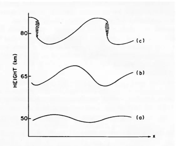
One of the more significant effects of gravity waves in the atmosphere is observed in the high-latitude mesosphere. During the winter months, when this region is predominantly in the dark, it is actually warmer than during the summer months when it experiences almost 24-hour sunlight. This seemingly counter-intuitive fact is due to the effects of gravity waves. Gravity waves propagating upward from their sources (generally in the troposphere) grow exponentially with height. This is due to the exponential decrease in atmospheric density; as these wave amplitudes grow larger, they become unstable and begin to break as illustrated in Figure 3.5. While the actual mechanics of gravity wave breaking are quite complex (Isler et al., 1994; Fritts et al., 1994; Andreassen et al., 1994) a simplified explanation will serve for the descriptive use of gravity wave breaking in this thesis.

(29)

3.4. Conclusion 25

Figure 3.5: Simple model of breaking wave breaking from (Andrews et al., 1987). breaking. Lindzen (1981) noted that the acceleration as a result of these breaking waves was more than sufficient to account for the mesosphere’s winter warming and summer cooling.

The process of summer cooling and winter warming works as follows; during the summer, the westward stratospheric jet causes westward-propagating waves to experience critical level filtering. However, eastward propagating waves will reach the mesopause where, as their amplitudes grow, they begin to break, transferring momentum to the background flow. This creates a eastward (or prograde) jet in the mesosphere, as well as a general eastward “body force” in the atmosphere in the region of breaking (Lindzen, 1981; Holton and Alexander, 2000; Garcia and Boville, 1994). Because the jet is moving in the prograde direction, it has excess angular momentum. To balance this, the air is forced away from the pole while conservation of mass requires it to be replaced by air from below. In the winter hemisphere the opposite effect occurs; the eastward stratospheric jet filters out eastward propagating waves, enabling westward waves to break in the mesosphere. This produces a westward jet with insufficient angular momentum, and therefore air moves toward the pole where it displaces air downward. This results in a pole-to-pole circulation.

The vertical motion of air in the summer hemisphere results in adiabatic cooling as the air parcel is expanded. This results in the cold summer mesosphere while the downward motion of air near the winter pole results in adiabatic compression and hence heating.

3.4 Conclusion

[image:29.595.177.459.58.292.2]

(30)

(31)

Chapter 4 MLT Gravity Wave Climatology

4.1 Introduction

This chapter develops a climatology of gravity waves in the Mesosphere Lower Thermosphere (MLT) using the Scott Base MF-radar data described in the previous chapter. Gravity waves propagating up from the lower atmosphere are acted upon by the wind field on their way to the MLT. These background winds can result in critical level filtering when their velocity vector matches the horizontal phase speed and propagation direction of the gravity waves. The filtering effects can be modelled by an atmospheric transfer function. The observed MLT gravity wave climatology can be used to examine the parameters required to derive a realistic atmospheric transfer function.

The climatology is produced using the Scott Base MF-radar measurements of the zonal and meridional winds between 70 and 96km. The wind data is composed of several signals; these include the mean wind speed and perturbations associated with long period atmo-spheric waves, such as the diurnal and semi-diurnal waves, as well as atmoatmo-spheric gravity waves. Removing all long period waves and long term trends from the wind data leaves only the wind perturbations associated with gravity waves and some instrumental noise.

Assuming that the noise is small, the kinetic energy per unit mass is calculated using the zonal and meridional wind perturbations. This energy is used as the gravity wave climatology for the year. Averaging several years together produces the overall gravity wave climatology.

4.2 Methodology

The techniques used to process the MF-radar data and develop a gravity wave climatology are common in the literature (see Vincent and Fritts, 1987; Dowdy et al., 2007). This thesis models its method on that found in Hibbins et al. (2007). However, it should be noted that while theHibbins et al.(2007) study bins the radar data at two-minute resolutions, this was not done in this study in order to reduce the computational overhead of the method.

Initially, the radar data was placed into 26 bins from 70 - 96km, the data region dic-tated by the radar data acquisition and high signal-to-noise ratio. All winds greater than

(32)

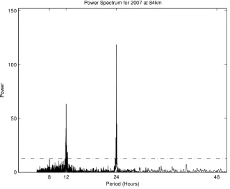
Figure 4.1: The wave periods present in the radar wind data in 2007. The dashed line is the 99% significance level.

100ms−1 _{were discarded at this point in order to remove the occasional artificially large}

wind measurement due to errors in the FCA algorithm. (Chapter 3.2.1). Note that while there is some radar wind data below 70km, the very weak D-region during the polar night means that the data availability is too low to be of use. The last height bin was selected to be 96km; above this altitude, ionisation becomes increasingly strong and electromagnetic effects become important (Fraser, 1984b). These electromagnetic effects mean that the as-sumption that the diffraction pattern observed by the radar moves due to the neural wind is likely to be violated. Furthermore, as height increases above 90km, very strong reflections from the E-region of the ionosphere can contaminate winds measurements, producing false winds (Hocking, 1997; Namboothiri et al., 1993)

Long period waves, such as the diurnal, semidiurnal and terdiurnal waves, often dominate the velocity field and therefore need to be removed to obtain wind perturbations from gravity waves alone. This was done by least square fitting a set of known period waves to the data and then removing them from each height bin. The periods of the waves to be fit were determined using a Lomb-Scargle periodogram (Figure 4.1). This gave strong peaks at 12 and 24h, and a weaker peak at 8h. These periods correspond to the diurnal, semi-diurnal and terdiurnal waves which would be expected to be present in this region.

[image:32.595.111.443.60.333.2]

(33)

4.2. Methodology 29

Figure 4.2: Example of radar gravity wave energy quality control

the day in the centre of a given five-day sliding window was not considered in the analysis. The equation used in the least squares fitting routine used in this analysis to remove the long period waves is shown below

y = Acos(−ω24t) +Bsin(−ω24t) +Ccos(−ω12t) +Dsin(−ω12t)

+Ecos(−ω8t) +Fsin(−ω8t) +Gt+H) (4.1)

where ω24, ω12, ω8 are the frequencies of the diurnal wave, semi-diurnal and terdiurnal

waves respectively;GtandH are the linear trend and DC offset; A−H are the least squares fit parameters. For example Acos(−ω24t) +Bsin(−ω24t) makes up the diurnal wave.

Each five day window the waveform of the long period waves was reconstructed from the least squares fit parameters and then subtracted from the radar data. The variance of the residual was then taken giving u02 _and _v02_{. It was assumed that this variance was due to}

gravity waves and some noise component. An additional quality control step was performed at this point to ensure that there were at least three data points in each least squares fitting set (per hour), and that they were less than two standard deviations away from a 15-day sliding mean over of the variance. Assuming a lognormal distribution, the variances were then reduced to daily means, which served to mitigate the effect of any white noise present.

The kinetic energy per unit mass is given by:

Ekm =

1 2(u

02₊_v02₎ _(4.2)

Taking the mean of the Ekm across a set of years yielded the gravity wave climatology

[image:33.595.153.480.57.323.2]

(34)

Figure 4.3: Averaging the gravity wave kinetic energy for each height bin and year.

It was particularly important to consider the quality of the radar data, as the MF-radar had undergone a substantial upgrade early in 2004. The upgrade involved a change to the radar control and data acquisition (Baumgaertner et al., 2006). This resulted in a significantly higher rate of data acquisition: in early 2004, the usual time between sampling periods was around eight minutes, while in early 2005 the system was collecting data at one set per minute. To test the effect of the upgrade, the gravity wave field was calculated for each year from 1985 to 2008, averaged across the whole year for each height bin taken. Figure 4.3 shows that after 2005 there was a large increase in the mean kinetic energy per unit mass, particularly at higher altitudes. For this reason, the final gravity wave climatology was generated using only data from 2005 to 2008.

In order to ensure that the climatology produced over such a short timespan was repre-sentative, an additional climatology was produced for the period from 1985 to 2004. While the magnitudes of gravity wave structures could be expected to differ because of the radar data acquisition upgrade, a broad similarity in the structures themselves would add credence to the 2005 to 2008 climatology.

[image:34.595.113.437.59.315.2]

(35)

4.3. Results and discussion 31

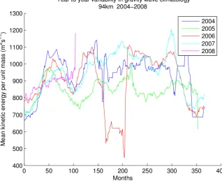
Figure 4.4: An early analysis of the variations in gravity wave energy between the years of the climatology revealed and anomalous section of data in 2006.

4.3 Results and discussion

The gravity wave climatology produced using MF-radar data between 2005 and 2008 is shown in Figure 4.5. It shows a general increase in gravity wave energy with height, due to gravity waves growing as the atmospheric density drops. The gravity wave field also shows strong seasonal patterns: during the Southern Hemisphere summer months there is generally less gravity wave activity than during the rest of the year. This is particularly apparent at altitudes below 85km where the gravity wave kinetic energy per unit mass is particularly weak around the equinoxes.

Since producing a climatology spanning a little over three years is potentially statistically unreliable, a climatology spanning 1985 to 2004 was also produced. While the magnitude of the pre-2005 climatology (Figure 4.6) is lower than the post-2005 climatology (particularly at higher altitudes), its overall structure is similar to that shown in Figure 4.5. This structural similarity increases confidence that the 2005-2008 climatology is not composed of a set of anomalous years, and that the radar accurately observes gravity wave fields.

[image:35.595.156.475.65.324.2]

(36)

Figure 4.5: Gravity wave climatology derived from the Scott Base MF-radar over 2005 to early 2008. Derived from variances of the wind residuals after removing tidal components. Smoothed with a 10% sliding window.

(37)

4.3. Results and discussion 33

Figure 4.7: Climatology of monthly mean wind variances between 1997 and 2005 at Rothera, from Hibbins et al. (2007). These wind variances are taken to be associated with gravity wave activity.

summer gravity wave energy observed in this region. The lower gravity wave energy in the summer mesosphere could also be due to gravity wave filtering by the atmospheric transfer function, preventing the gravity waves from reaching the region examined by the MF-radar. The rapid increase in gravity wave energy observable at 74-76kmin Figure 4.5 could also be due to the formation of the polar night jet at this time of year. This has been shown to generate gravity waves, possibly as a result of geostrophic adjustment around the jet (Sato, 2000; Sato et al., 1999).

(38)

Figure 4.8: Climatology of zonal and meridional wind variances after removal of tidal com-ponents at Davis (top panel) and Syowa (bottom panel). Adapted fromDowdy et al.(2007).

(39)

Chapter 5 Radiosonde Derived Gravity Wave

Source Function

5.1 Introduction

Gravity waves propagating from the lower atmosphere are modified by various processes, such as critical level filtering and gravity wave breaking. The integrated effect of these processes can be modelled by an atmospheric transfer function. This transfer function can be multiplied by a source function – a measure of the wave activity variation associated with sources alone – to produce a simulation of the high altitude gravity wave field discussed in the previous chapter. This chapter seeks to determine an empirical source function for gravity waves based on radiosonde observations from balloons launched from McMurdo Base, Antarctica.

Using established techniques, the kinetic and potential energy associated with gravity waves were calculated at a variety of altitudes over the period from 2000-2007. The sum of the potential and kinetic energy is referred to as the total gravity wave field. The gravity wave source function is calculated over a variety of altitudes in the troposphere and over the tropopause/lower stratosphere. Analysing the interaction of the source functions with the atmospheric transfer function should provide insight into the contribution of low altitude gravity wave variability to the high altitude (75-96km) wave field. For example, if the filtered source function displays a low correlation to the observed gravity wave climatology, this could indicate that waves were being generated at higher altitudes, or that gravity waves were moving horizontally into the observation area. Finally, crude gravity wave phase direction information can be obtained by fitting ellipses to hodographs of wind changes with altitude.

5.2 Methodology

Gravity waves in the troposphere can be produced in several ways (see Section 3.1.1). The primary mechanisms are: flow over mountains, shear generation, geostrophic adjustment

(40)

and deep convection (Fritts and Alexander, 2003). Since the Antarctic is too cold for any significant convective activity, the last source can be omitted from this discussion.

The gravity wave source function was calculated using data from radiosondes launched at McMurdo Station, which is approximately 1.5km south of the receiving antennas at Arrival Heights. It can therefore be assumed that these radiosonde observations are indicative of atmospheric conditions similar to the Arrival Heights MF-radar, though obviously they examine different altitude ranges.

The source functions are defined by the gravity wave field in the troposphere and in the stratopause. The gravity wave field is obtained from wind velocity vectors and temperature measurements sampled by radiosondes as they rise through the air column. Calculations of gravity wave activity measures are completed using well-established methods discussed in Vincent and Alexander (2000) and Tsuda et al. (2004). Briefly, the radiosonde data is placed into altitude bins in order to be consistent between successive flights. After binning the data, a second order polynomial is fitted to the temperature profile and wind speeds in the zonal and meridional directions. This polynomial is subtracted from the raw data in order to obtain the gravity wave perturbations around the mean.

The gravity wave field is then given by the sum of the kinetic and potential energy per unit mass at each altitude bin. The relevant equations are

Ek =

1 2

u02+v02 (5.1) where Ek is the kinetic energy per unit mass, and u0 and v0 are the zonal and meridional

components of the perturbation velocities. Note that the vertical component of the kinetic energy is ignored, as it is considered too small to be of significance (Yoshiki and Sato, 2000).

The potential energy per unit mass(Ep) is calculated using

Ep =

1 2

_g

N

2 _T0

T0 !

(5.2) where T0 is the temperature perturbation; T0 is the mean temperature profile as measured

by the radiosonde; g is gravitational acceleration, and N is the Brunt-Väisälä frequency, which (following Andrews et al. (1987)) is given by:

N2 = g

T

Ts

∂lnθ

∂z = R H ∂T ∂z + κT H ! (5.3) The termsT andTsare the temperature with respect to altitude and surface temperature

respectively; g is the acceleration due to gravity; R is the gas constant for air; θ is the potential temperature; H is the scale height, which varies from 6km in the troposphere to roughly 7km in the stratosphere; κ ≡ R/cp ≈ 2/7 where cp is the specific heat at constant

(41)

5.2. Methodology 37

Figure 5.1: McMurdo radiosonde sampling altitude statistics between 1 and 8km. Each balloon flight between 2000 and the start of 2007 is displayed. The average difference in altitude between measurements is displayed, as well as the maximum and minimum difference for each flight.

The kinetic and potential energy are calculated for each radiosonde flight. The energies are then converted to daily averages assuming a lognormal distribution.

Ideally to obtain gravity wave data, high vertical resolution data should be used (Vincent and Alexander, 2000). Tsuda et al. (2004) use 100m vertical resolution data, while Vincent and Alexander (2000) and Yoshiki and Sato (2000) use 50m binning. In order to determine the altitudes for the McMurdo radiosonde data, the average difference between successive altitudes in the raw data ∆zis plotted for each flight in the measurement period between 2000 and 2007. Figures 5.1 and 5.2 show that the quality of data available varies quite substantially before and after mid-September 2004. The value of ∆z prior to this date is roughly 175m, while afterward the average difference is less than 15m.

[image:41.595.156.481.56.328.2]

(42)

Figure 5.2: Another way of examining the radiosonde’s data sampling is to calculate the least squares linear slope of differences in height vs. sample number.

While the increase of ∆z with height prior to the upgrade is fairly small, the fairly coarse vertical scale will remove part of the gravity wave spectrum. Ideally, this would mean that only data after 2005 should be used. However, the McMurdo radiosonde data is currently unavailable after 31st of March 2007, which leaves only two years of data. This may be insufficient to be representative, particularly in light of the likely variations in the gravity wave field over several years. Therefore, data from 2000 to 2007 is used and binned every 200m, as this is the average distance between height measurements for the pre-2005 McMurdo radiosonde data (see Figure 5.1).

Binning the radiosonde data every 200m introduces an observational filter to this data, removing small vertical wavelength gravity waves (Alexander, 1998). For this reason, com-plementary source functions are produced with a 40m binning. However, these will only be produced after September 2004, when the data quality becomes sufficient to justify this resolution. The data binned at 200m will be used to verify that the climatology produced with 40m altitude resolution is reasonable.

Climatologies are produced over two altitude ranges:

• from 1−8km(within the troposphere), the region in which gravity waves, particularly topographic gravity waves, are generated;

[image:42.595.111.443.55.332.2]

The Atmospheric Gravity Wave Transfer Function above Scott Base

Department of Physics and Astronomy, University of Canterbury,

Private Bag 4800, Christchurch, New Zealand