A meteor orbit radar

(1)

A

METEOR ORBIT RADAR

A

THESIS

SUBMITTED IN PARTIAL FULFILMENT OF THE REQUIREMENTS FOR THE DEGREE

OF

DOCTOR OF PHILOSOPHY IN PHYSICS IN THE

UNIVERSITY OF CANTERBURY

BY

Andrew D. Taylor

(2)

(3)

PHYSICAt: SCIENCES

LIBRARY THESIS

Abstract

A Meteor Orbit Radar, AMOR, has been built near Christchurch, New Zealand. It uses a narrow beam pulsed radar to detect meteors down to a

+

12.5 radio-meteor magnitude limit. AMOR measures the relative timelags between the onset of meteor echoes at each of three spaced receiver stations to calculate the meteoroid velocity with an accuracy of ±2.5 km.s-1

. A 'Luggable' MAC

AT is used to run the radar, identify meteor echoes and record raw observation records.

A total of 1.3 X 105 meteor velocities have been determined using the new timelag method. For 1.6 X 104 _{of these observations velocity measurements}

could be made using Fresnel diffraction patterns and these were in complete agreement with those from the new timelag velocity technique. The diffraction patterns recorded by AMOR allow atmospheric decelera.tions to be determined by calculating the velocity for overlapping subsections of the patterns. Typi-cally, the atmospheric decelerations found lay between 0 and 40 km.s-2 •

Observed meteor velocities need to be corrected for the presence of the Earth before a heliocentric meteoroid orbit can be calculated. AMOR uses a new vector scheme to make corrections for atmospheric deceleration, the rota-tion and gravitarota-tional accelerarota-tion of the Earth, conversion to a heliocentric frame using rotation matrices and a correction for the orbital velocity of the Earth. This new derivation greatly simplifies the theoretical framework for computer based calculation of meteor orbits.

The 1990 apparition of the

r;

Aquarid meteor shower was used as a calibra-tion test for the complete AMOR system. 270 shower meteors were detected giving a mean stream orbit with elements of q = 0.57AU, e

=

0.98, i

=

165.5°,

w

=

97°,

n

=

46°. This agrees closely with previous orbits given for the

r;

Aquarid stream and demonstrates the very large improvement in meteor stream characteristics that can be achieved by AMOR. Orbital elemel'tts for individual

r;

Aquarid meteors can be determined within the following mea-surement limits: 0.33

<

q

<

0.76 AU, 0.76

<

e

<

1.45, 163.0°

<

i

<

167.5°, 62°

<

w

<

126°, 35

<

n

<

49°.

(4)

(5)

List of Tables

1.1 Review of Previous Orbit Radars 7

2.1 History of the Receiver Arrays 24

4.1 System Time Delays

...

76

4.2 Timelag Comparisons

...

106

4.3 Comparison of Timelag Examples . 127

7.1 AMOR TJ Aquarid Observing History . 196

7.2 Station Data Measurement Uncertainties . 213

7.3 Orbital Element Uncertainties . 214

7.4 TJ Aquarid Orbital Elements . . . 242

8.1 Days in Heliocentric Radius Bins 247

8.2 Corrections to Observed Velocity 2(:)8

8.3 Summary of AMORT] Aquarid Orbits 269

(12)

(13)

List of Figures

2.1 RF Layout of the AMOR System . . . . 2.2 26.2 MHz AM Receiver Circuit Diagram 2.3 Receiver Bandpass Curves . . . . 2.4 Receiver Calibration Curves . . . . 2.5 Home Site Receiver Calibration Curves . 2.6 Schematic Layout of Collinear Receiver Array . 2.7 Theoretical Receiver Antenna Gain Patterns. 2.8 Early Receiver Array Power Distributions . . . 2.9 Collinear Array Power Distribution . . . . 2.10 Schematic Layout of Rhombic Transmitter Array 2.11 Transmitter Array Power Distributions .

2.12 Example of VCO Non-Linearity . . . . 2.13 Calibration Curves with VCO problem

3.1 Observation Software Layout . . . . 3.2 Observation Program Memory Map. 3.3 SweepBlock Data Array

3.4 Observation Record 3.5 Detection Information

4.1 Schematic for Range Timing . 4.2 Radar Station Layout . . . . 4.3 Peak Amplitude Range Offsets 4.4 DeSpiking Amplitude Profiles . 4 . .5 Despiking Severe Corona . . . .

4.6 Triangular Amplitude Profile Smoothing . 4.7 Receiver Amplitude Range Scan

4.8 Calibration of Recorded Amplitude . 4.9 Recorded Ma.ximurn Amplitudes 4.10 Phase Angle Example . . . 4.11 Calibration of Phase Angle 4.12 Old Fit of Phase Angle . . 4.13 Phase Angle Distribution 4.14 Elevation Angle . . . .

(14)

4.15 Phase Range Distribution . . . . 4.16 Resolve Phase-Elevation Angle Ambiguities 4.17 Ionisation Height Distribution . . . . 4.18 Weather Log for Phase Angle Calibration 4.19 Example Observation for Timelag Calculations 4.20 Pre-Fresnel Interference ..

4.21 Delayed Rise To Ma..ximum 4.22 Profile Rise Points . . . . 4.23 Wind Blown Rising Edge 4.24 Maximum Rising Slope . . 4.25 Ambiguous Rising Edge

4.26 Full Profile Cross Correlation Profile 4.27 Cross Correlation Rising Edges . . . 4.28 Rising Edge Cross Correlation Profile 4.29 Poorly Placed Rising Edge Sections . 4.30 Poor Rising Edge CCF . . .

4.31 Echo Decay Slope . . . . 4.32 Delayed Exponential Decay 4.33 Small Amplitude Profile . .

4.34 Wind Shear Affected Decay Profiles 4.35 Home Site Diffusion Heights . . .

4.36 Comparison of Geometric and Diffusion Heights . 4.37 Reflection Geometry . . . . .

4.38 Unit Tangent Velocity Vector

5.1 Mean Amplitude Profile .. 5.2 Find Relative Phase Angles 5.3 Meteor Deceleration . . . . 5.4 Atmospheric Deceleration

5.5 Fresnel Atmospheric Decelerations 5.6 Rapid Atmospheric Decelerations .

5.7 Atmospheric Deceleration Velocity Dependence 5.8 Comparison of Timelag and Fresnel Speeds 5.9 Hyperbolic Meteoroids . . . .

5.10 Ecliptic Projection of Hyperbolic velocities

6.1 Orbital Motion in Polar Coordinates 6.2 Rotational Velocity of the Earth . . . 6.3 Gravitational Attraction of the Earth 6.4 Rotation of Bin x-y Plane . . . . 6.5 Rotate Coordinates to North Celestial Pole 6.6 Convert to Equatorial Coordinates

6.7 Convert to Ecliptic Coordinates . . . 6.8 Convert to Heliocentric Coordinates

(15)

LIST OF FIGURES

6.9 The Orbital Motion of the Earth . . . . 6.10 Heliocentric Position and Velocity of the Meteoroid . 6.11 Orbital Motion of a Meteoroid

XV

185 188 190

7.1 TJ Aquarid Radiants. . . 199

7.2 Daily Motion of TJ Aquarid Radiant . 200

7.3 TJ Aquarid Heliocentric Velocities 202

7.4 Sporadic Radiants . . . 203

7.5 . Observed TJ Aquarid Velocities. 204

7.6 1990 May 4 Meteor Radiants . 206

7.7 Daily Motion of Radiant . . . . 208

7.8 TJ Aquarid Orbital Elements - Shape 209

7.9 TJ Aquarid Orbital Elements - Orientation 210

7.10 Orbital Element Measurement Uncertainties- Shape 216

7.11 Orbital Element Measurement Uncertainties- Orientation 217

7.12 Total Observations 1991 April 28 to May 18 . 218

7.13 Total Element Distributions - Shape . . . 220

7.14 Total Element Distributions - Orientation 221

7.15 Non Shower Inclinations .. 7.16 Inclination- Velocity

7.17 D-Criteria Stream Members 7.18 Serial Search DD Stream Members 7.19 D-Criteria 17 Aquarid Elements - Shape 7.20 D-Criteria 17 Aquarid Elements- Orientation 7.21 Meteoroid Orbit Element Density Cross-Sections 7.22 Heliocentric Velocity Components . . . . 7.23 D-Criteria Orbit Population Cross-Sections 7.24 TJ Aquarid Stream Search ..

7.25 Comet Halley Stream Search 7.26 Radiant Clumps . . . .

8.1 Perihelion Distance from the Sun 8.2 Observed Atmospheric Meteor Speeds

8.3 Ecliptic Projection of Heliocentric Velocities . 8.4 Components of the Bimodal Velocity Distribution . 8.5 Argument of Perihelion Distribution . . . . 8.6 Prograde and Retrograde Perihelion Components 8.7 Prograde and Retrograde Perihelion Distances . 8.8 AMOR Observation and Orbit

8.9 Fresnel Diffraction Patterns . . . . 8.10 Hyperbolic Orbit . . . . 8.11 Small Amplitude Meteor Observation

8.12 TJ Aquarid Radiants Before and After AMOR

(16)

D.1 Perihelion Distance . . . 412

D.2 Orbital Eccentricity . . . . 412

D.3 Inclination of Orbital Plane 413

D.4 Argument of Perihelion . . 413

D.5 Longitude of the Ascending Node . 414

D.6 Inverse Semi-Major Axis . 414

D.7 Semi-Major Axis . . . 415

D.8 Log Semi-Major Axis . 415

D.9 Aphelion Distance . . 416

D.10 Log Aphelion Distance 416

D.ll Observed Atmospheric Speeds . 417

D.12 Fresnel Diffraction Speeds . . 417

D.13 Corrected Geocentric Speeds . 418

D.14 Heliocentric Speeds . . . 418

D.15 Ecliptic Projection of Heliocentric Velocity 419

D.16 Home Site Echo Amplitudes . 420

D.17 Home Range to Meteor . . 420

D.18 Nutt Site Echo Amplitudes 421

D.19 Nutt Range to Meteor . . . 421

D.20 Spit Site Echo Amplitudes . 422

D.21 Spit Range to Meteor . . . 422

D.22 Geometric Height of Home Site Reflection Point 423

D.23 Diffusion Height of Home Site Reflection Point 423

D.24 Geometric Height of Nutt Site Reflection Point 424

D.25 Diffusion Height of Nutt Site Reflection Point . 424

D.26 Geometric Height of Spit Site Reflection Point 425

D.27 Diffusion Height of Spit Site Reflection Point 42.5

D.28 Elevation Angle, Polar Plot . . . 426

D.29 Relative Home Site Phase Angle 426

D.30 Tin Phase Amplitudes . . . 427

D.31 Tos Phase Amplitudes . . . 427

D .32 Comparison of Timelag and Fresnel Speeu.., 428

(17)

Chapter

1

Introduction

1.1

Interplanetary Dust and Meteors

A considerable amount of material orbits the Sun between the planets. The larger objects like asteroids and comets can be viewed directly from Earth, while objects smaller than several hundreds of metres across cannot be re-solved individually even by powerful telescopes. Dense concentrations of small particles, such as the rings of Saturn, can be seen en masse. Similarly, sunlight reflected from the very small particles, a few tens of microns in size, in orbit around the Sun produces a faint glow which can be seen as the zodiacal light. The presence of objects between these sizes can be inferred when they collide with other bodies. Impact craters on the Moon and micropits on spacecraft are examples of such evidence. More spectacularly when particles hit the at-mosphere of the Earth they produce meteors. Very bright ionisation trails, often called fireballs,. are associated with a meteorite that survives to hit the Earth. Smaller particles, down to zodiacal dust size, ionise completely in the atmosphere. Both wide angle cameras and television systems have been used to detect faint meteors th? ', cannot be seen by the unaided human eye. Very faint meteor trails can be ttetected by more powerful radars.

Most of the particles detected as meteors are believed to have come from comets. Each time a comet approaches the Sun, at perihelion, it is heated by solar radiation. The volatile components near the surface are evaporated and ejected from the comet. The solar radiation ionises the gas to a plasma and then blows it away on the solar wind forming a gas tail streaming from the comet. Dust particles are dislodged from the comet as the gas evapo-rates from the surface. The very smallest, less than one micron, of these are also accelerated by the solar wind and form a distinctive dust tail or fan. Larger particles remain in much the same orbit as the parent comet. The small range of ejection velocities from the nucleus combined with subsequent gravitational perturbations by the planets spread these larger dust particles around the comet orbit forming an associated meteoroid stream. Close

(18)

tary encounters move some of these stream particles into random or sporadic orbits. Various radiation effects change the particle orbits more slowly. Inter-planetary collisions between particles shatter the dust producing a range of fragment sizes. Remnants smaller than about one micron are accelerated by the solar wind and blown out of the Solar System.

As the Earth moves around its orbit a tiny fraction of this interplanetary dust complex will hit the atmosphere. By observing the ionisation trail as it forms behind a meteor it is possible to measure the particle velocity. From this, the heliocentric meteoroid velocity can be calculated and hence the orbit of the interplanetary dust particle. Observations of meteor orbits can be used as a probe for the distribution and dynamical characteristics of interplanetary dust.

An orbit radar has been built at Christchurch, New Zealand to observe meteors and calculate the associated meteoroid orbits. This installation, A Meteor Orbit Radar (AMOR), is the subject of this thesis.

The radar is expected to give a greatly increased volume of orbit data on major meteors streams. This will provide a greater statistical base on which to base mean orbits for the streams. For example the mean orbit given for the

77 Aquarid stream in the list of streams by Cook

et

al (1972) is based on one

observation. The order of magnitude increase in data should make it possible to investigate fine structure in these major streams.

The AMOR system is capable of detecting meteors to a radar magnitude limit of +12.5 to +13 thereby observing particles down to a size of about

100 J-lm. The distribution of the orbital element for sporadic meteors in this

size range is of interest in understanding its potential as a reservoir of material to form the zodiacal dust cloud.

Radar reflections from meteors can be used as a probe to study the struc-ture and motion of the atmosphere. The diffusion and body motion of the ionisation trail in the neutral atmosphere allows for making measurements of density and wind velocities to be made. Knowledge of the orientation and track of the particle forming the ionisation trail provides useful extra informa-tion in studies of this kind.

Over 100 asteroids that cross inside the orbit of the Earth have been dis-covered. This group of minor planets is divided into three classes named after the first such object discovered. The Apollo asteroids cross inside the orbit of the Earth with a perihelion distance of less than 1.017 AU. Aten aster-oids form a subset of this group with an orbital semi-major axis of less than 1.0 AU. Amor asteroids have a perihelion distance of less than 1.3 AU but do not cross inside the orbit of the Earth. There are too many asteroids in this Apollo-Aten-Amor complex for the group to be dynamically stable. Close encounters with planets would cause them to be ejected from the inner Solar System in times that are short compared with the age of the Solar System.

(19)

diffi-1.2. VISUAL METEOR OBSERVATIONS 3

cult. Deactivated comets have been suggested as a candidate source. If these asteroids were once comets they are likely to have meteoroid streams associ-ated with them. For those asteroid orbits which intersect with the orbit of the Earth these cometary fingerprints should be evident amongst the meteor orbit distribution. One of the primary motivations for developing the Christchurch radar was to search for meteor streams associated with near Earth asteroids. The AMOR acronym is doubly appropriate.1

1.2

Visual Meteor Observations

In the later part of the 19th century the importance of acquiring orbital infor-mation on meteors was recognised by Schiaparelli and Newton. Some indica-tion of meteor radiant and velocity distribuindica-tions of the meteoroid populaindica-tion can be achieved from observations of the diurnal, seasonal and latitudinal vari-ation of meteor influx. A quantitative model fitting approach along these lines was first considered by Schiaparelli (1866). It was later used by Hoffmeister ( 1948) for example to delineate crude orbital discriminations thought erro-neously to have a large interstellar component.

1.2.1 Visual Orbit Determinations

Denning (1899) and Prentice (1945) in Britain used angular velocity estimates of visual meteors in attempting to determine whether meteoroids were trav-elling in closed heliocentric orbits. Meteor trajectories were mapped using coordinates superimposed by the observer and angular velocities calculated by timing estimates.

The first precise quantitative information came from the rocking mirror de-vice of Shapley et al ( 1932). Ivleteor tracks were measured using a fixed reticle of hour angle and declination with angular velocity estimated by the rocking mirror. An observer watched the reflected meteor track. The pattern of loops together with height data. gained from simultaneous observations at stations separated by a 40 km baseline gave velocities. The field of view was 60° and meteors down to +4 magnitude could be recorded. For fainter meteors the rocking mirror could be used in conjunction with 4 inch reflecting telescopes. The main emphasis of this work carried out during the Harvard-Cornell Ari-zona. Meteor Expedition 1931-3 was in securing geocentric velocities. This visual survey concluded that about 60% of sporadic meteors had velocities exceeding the parabolic limit ( Opik, 1948).2

1

0f course any PhD thesis turns into a work of love at some stage and AMOR seemed

appropriate in this sense as well. I discovered the word while at the First Vatican Summer School (1986) in Astronomy and Observational Astrophysics, hence the Latin or Italian spelling.

2

(20)

1.2.2 Photography

More objective records started with the application of photographic techniques to meteor observations. Some of the earliest meteor photographs were obtained on the Harvard photographic patrol programme in the 1890s.

The use of separated cameras with occulting shutters over their lenses to give angular velocity was first employed by Elkin (1899) at Yale in the U.S.A. 1894-1909. The system baseline of only 3.5km limited the resolution obtained on the 131 photographic tracks later analysed by Olivier (1937). Improvements in emulsions and cameras allowed for a long programme at Harvard initiated by Fisher and Olmsted (1929) and continued by Millman. From 1936 the programme continued under Whipple who was able to derive atmospheric density values from measured meteor decelerations.

The cameras employed in these surveys were only sensitive to meteors brighter than magnitude -1. With their angular field of 60° the acquisition rate was only 1 per 100 observing hours. This limitation of only a handful of orbits over the years of operation was overcome with the Super Schmidt cameras (limiting magnitude +4) operated by Harvard University at Soledad Canyon and Dona Ana in New Mexico. 2800 orbits were secured in the period 1952-9.

Other multi-station camera determinations of orbits has been carried out at Dushanbe, 197.5-83; Ondrejov Observatory (Czechoslovakia) 1951-86; Odessa and Kiev. Much of the published Super Schmidt orbit results appear in the Smithsonian Contributions to Astrophysics series of publications (for example Vol4 no 2 and no 4, 1961). More recently photographic observations of meteor orbits have been continued by amateur groups using 35mm rotating shutter spaced cameras in Netherlands (Beltlam and de Lignie, 1989) and in Japan (Koseki, 1989).

Orbits of fireballs have been secured by fisheye camera networks. The Prairie network in the U.S.A. under the direction of the Smithsonian Institute operated in the period 1963-75. The European Network of Central Europe with 52 stations (as of 1990) in Czechoslovakia, Germany and Netherlands has continued to produce orbits from 1964 to the present. The Meteorite Observation and Recovery Project (MORP) has operated in Canada from 1971. Meteor orbits from MORP are presented by Halliday et al (1983) and (1989).

1.2.3 TV Cameras

(21)

1.3. RADAR ORBIT MEASUREMENT TECHNIQUES 5

sec angular accuracy. This translates to an accuracy in the orbital elements of± 1-2°, with the eccentricity accurate to about ±0.0.5.

1.3

Radar Orbit Measurement Techniques

Some information on the radiant distribution of meteors can be gained by mak-ing use of the specular reflection property of the radio scattermak-ing process from

an ionised column. A statistical approach using occurrence-time and radar range-time characteristics obtained using a radar with antennas of known an-gular response was proposed by Clegg ( 1948). This was used at Jodrell Bank to isolate shower radiants and to deduce the sporadic radiant distribution over the celestial sphere. A combination of radiant coordinates obtained from this statistical method together with velocity information (section 1.3.2) permitted the determination of a representative shower orbit.

To determine the heliocentric orbits of individual meteors it is necessary to locate the radiant and hence the direction of the meteor trajectory and the pre-atmospheric velocity for the particle. The actual position ofthe ionised column in space with respect to the Earth is not actually required. Essentially three receiving stations as first proposed by Kaiser (Hawkins, 1964) are required.

Three principal methods have been employed for the determination of in-dividual meteor orbits.

1.3.1 Range-Time

The reflection process of the radar echo from the main body of the ionisation trail is one of specular geometry. The echo strength is clue to the contributions of several Fresnel zones on either side of the specular point. However. for very bright meteors the body echo is often accompanied by a head echo. This seems to be associated with a ball of ionisation travelling with the meteoroid in front of the developing ionisation column (Simek, 1973). A range- time plot of the reflections from this plasma ball will describe a hyperbola from which the atmospheric velocity of the particle can be measured. The first such determination was by Hey and Stewart (1947) in their measurement of velocities for the Giacobinicls during the 194 7 apparition. Three station range-time comparisons yielded the meteor location and trajectory. This method can be used only for very bright meteors producing intense ionisation.

1.3.2 Pulsed Radar

(22)

each Fresnel zone successively adds in and out of phase thereby adding and subtracting to the amplitude of the signal. The period of these oscillations in the diffraction pattern permits the atmospheric velocity of the meteor to be determined. Modifications to the ideal straight edge function due to diffu-sion, meteor deceleration and wind shear have been considered, for example by Southworth (1972). The first measurement of a meteor velocity using this technique was reported by Ellyett and Davies (1948). Employing three spaced stations will yield three diffraction patterns. A separation of about 5 km be-tween the receiver sites ensures that the reflection points on the meteor trail are separated by a small distance compared with the overall length of the ionised column. Timing differences in the occurrence of the echo profile at each site each gives the direction of the trajectory. Ranges to the meteor trail are measured by pulse timing.

A coherent phase system can be added to the pulsed radar. By providing a reference signal to the receiving sites, Doppler measurements of the atmo-spheric wind can be made and then wind effects allowed for in data reduction. The presence of a reference phase makes it possible to measure oscillations in the diffraction pattern as the meteoroid approaches the specular reflection point. The pattern continues symmetrically after the point of closest approach.

1.3.3 Continuous Wave Technique

A CW radar measures the differential phase between the reflected signal and the transmitter ground plane reference. The transmitter and receiving stations need to be separated by some tens of kilometres to reduce interference. This phase information is used to calculate the direction of arrival at each of several, but a minimum of three, receiving sites. Direction cosines to the meteor from each receiver site can be determined. Additionally the coherent phase CW operation permits measurement of the fluctuations due to Fresnel zones formed both before and after the meteor particles motion through the specular reflection point. This has the advantage of being less affected by trail distortion and diffusion effects.

1.4

Review of Previous Orbit Radars

McKinley and Millman (1949) extended the range-time dependence of head echoes to three stations using omni-directional antennas to determine a few orbits. Being limited to very large meteors the successful orbit rate was only about 1 per 100 hours of observing. Manning et al (1948) and McKinley (1961) used CW systems with photographic recording of a single frame triggered camera.

(23)

1.4. REVIEW OF PREVIOUS ORBIT RADARS 7

Location Dates of Number of -Limiting Reference

Operation Orbits magnitude

Ottawa 1948 McKinley and Millman (1949)

Stanford 1948 Manning et al (1948)

Ottawa 1950 McKinley (1961)

J odrell Bank 1954- 1955 2509 +8 Davies and Gill (1960)

Khankov 1960- 1966 12,500 +7 Le bedinec ( 1968)

Adelaide 1961 2092 +6 Nilsson (1964)

Havana 1961 - 1969 40,000 +12 Cook et al ( 1972)

Kasan 1968 1200 +8 Andrianov et al (1970)

Adelaide 1968 - 1969 1667 +8.5 Gartrell and Elford ( 1975)

Table 1.1: Review of Previous Orbit Radars

transmitter antenna beam 24° wide with a gain factor of 28 was used in con-junction with spaced receiver stations with aerial gains of 12 which were sep-arated by 3.5 km baselines. Photography of amplitude-time displays recorded the data and orbit determinations were attempted on selected echoes showing at least three diffraction zones.

Nilsson (1964) ran a combined CW and pulsed system with four outsta-tions. The transmitter was separated by 20 km to reduce the amplitude of the ground pulse. The transmitter operated on 27MHz and produced 10kW pulse with 300 watts CW. The aerial system used a vertical 3 element Yagi for the transmitter and half wave dipoles a quarter wavelength above ground for the four receiver stations. The resultant power distribution was omnidirectional in azimuth and broad in elevation with a maximum to the zenith. The system produced on average 1.3 orbits per hour of observing. Reduction of signals was accomplished by photography of displays, filmreader to punched tape and finally to punch cards. The update reported by Gartrell and Elford ( 197.5) employed a 65 kW pulse at 200Hz on 27.5 MHz. with 26.8 MHz 1.5 kW CW and six outstations.

(24)

well defined echo amplitude fluctuations for fast meteors a high pulse frequency of greater than approximately 600Hz is necessary thus introducing aliasing in range measurement. Fragmentation produces multiple sources damping out the resultant Fresnel pattern while wind distorts the profile. Davies and Gill state that only 10% of echoes in their survey were useable. In the present AMOR radar we find approximately 4% yield simultaneous diffraction patterns from 2 or 3 receiver stations while approximately 10% give a pattern on one. Routine velocity measurement in AMOR does not use diffraction patterns but rather times the intervals between the appearance of the echo profiles on spaced receivers. However Fresnel velocities do provide an important calibration.

Orbit determinations of very faint meteors have been achieved in general by substantially increasing the transmitter power. Building a 2 MW transmitter similar to that used in the Havana radar is a very difficult engineering exercise. The same increase in magnitude can be achieved by increasing the antenna gain with some sacrifice in angular coverage at any one time. This approach is used by the Christchurch AMOR system to reach a limiting magnitude of +12.5 with a 20 kW peak power pulsed transmitter.

Previous orbit radars have used photography of oscilloscope displays to record the data. The film was developed, measured and reduced thus requir-ing a considerable labour in selectrequir-ing and measurrequir-ing appropriate observation records. More recently computers have been used to speed the calculation of orbits from this measured data. The Christchurch radar was conceived as a microprocessor based system with receiver output voltages converted directly to a digital amplitude. Several chains of microprocessor boards were designed and built giving a multichannel system that recorded radar information in a machine readable form for subsequent computer analysis.

1.5

Christchurch Meteor Orbit Radar

(25)

ac-1.5. CHRISTCHURCH METEOR ORBIT RADAR 9

cess to the AMOR data base.

A meteor orbit radar needs to locate the meteor in space and determine its velocity. Effectively six kinematic degrees of freedom need to be determined for the particle. As the meteoric particle is too small to be seen directly this is done by watching the associated ionisation trail formed in its wake. The

AMOR system uses a 26.2 MHz pulsed radio transmitter to detect meteoric ionisation trails. By timing the delay between the sending of a pulse and the detection of the meteor echo the range to the target trail can be determined thus fixing one of the positional degrees of freedom. Radar pulses are sent by the transmitter every 2.64 ms making it possible to determine unambiguous ranges to meteor trails out to about 400 km.

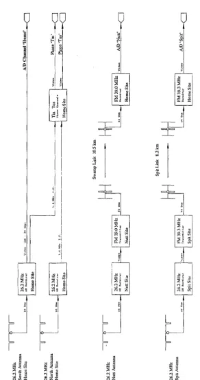
The Christchurch AMOR radar uses long broadside antenna arrays which concentrate the antenna gain in a narrow azimuthal beam with a 3° width. These beams are aligned to point north-south and hence locate the azimuth angle to the meteor trail. A rhombic transmitter array directs most of the radar power south making detection of meteors travelling from north of the station more likely. The antennas are suspended about 0.6.\ above the ground and produce a broad beam in elevation. Two spaced antennas at the Home site of the radar station act as an interferometer to determine the elevation angle of the returning echo. The range, elevation angle and implied azimuthal angle locate the meteor trail relative to the radar station.

AMOR uses a backscatter configuration to detect the meteor trails. The ionisation column formed by the meteor acts as a long thin reflector at the 11.45 m radar wavelength. To receive an echo at the radar station the trail must be at right angles to the radar beam. The particle must be travelling in a. plane normal to the direction of the received meteor echo. As the meteor moves past the specular reflection point the echo amplitude increases as the ionisation trail forms. The column then diffuses into the neutral atmosphere and the echo strength decays away. The echo amplitude associa.t.ed with each transmitter pulse is recorded by the system giving an amplitude profile with a. 379 Hz sample rate. By comparing the timelags between the rising edge sections of the echo profiles from three spaced receiver stations the final two components of the velocity can be determined. The two remote receiver sites are separated by 8.18 km and 10.54 km from the Home site.

The current philosophy behind the equipment design is to cligitise the radar data and insert it directly into the computer memory of an IBM PC-AT compatible as quickly as possible. Detection algorithms written in high level software are initiated by an interrupt every 2.64 ms to locate meteor echoes in the previous radar range sweep. From here the observation data necessary to calculate a meteor orbit can be extracted and stored. The time of occurrence, range, duration of the trail, three echo amplitude profiles and two phase angle profiles are recorded for each meteor observation. From this information the relative position and velocity of the meteor particle are calculated.

(26)

made and the position and velocity converted to a heliocentric reference frame. The orbit reduction package employed by AMOR to do this uses a new tech-nique based on vector notation for the meteor velocity. From this the orbital elements for the meteoroid's motion around the Sun are calculated.

1.6

AMOR Thesis Layout

This thesis discusses the meteor orbit radar developed at the University of Canterbury, Christchurch, New Zealand. It describes the radar hardware, ob-serving software and data reduction techniques. A new method for converting the observation data to a heliocentric orbit is developed. The Fresnel diffrac-tion method for determining meteor velocities is investigated as a check on the timelag based method used by AMOR. The 1990 observations of the TJ Aquarid meteor shower are used as an astronomical calibration of the radar.

The chapter on the radar hardware describes the main features of the radar installation. The performance characteristics of the 26.2 MHz radio frequency components are covered in addition to the phase comparison system of the Home site interferometer. The design and theoretical gain calculations for both the the transmitter and receiver aerial arrays give an estimate of the gain achieved. The work involved in checking the radiated power distributions and alignments for the arrays is highlighted. A limiting radar magnitude of+ 12 .. 5 is found for the AMOR system. The operation of the two FM data links from the remote receiver sites is described. The digital hardware which controls the radar and the operation of the direct memory accessing to get meteor echo data into the computer are both covered in Section 2.5. A brief historical note on equipment superceeded in the period 1978-91 is included.

The observation software runs the computer during an observing run. The associated data structures and memory use within the program are described. Every 2.64 ms an interrupt is sent from the control hardware and initiates the execution of a meteor detection routine. The assembly of the observation data record necessary for an orbit calculation is described. Finally in this chapter the temporary storage of observation records in extended memory and subsequent archiving is covered.

(27)

1.6. AMOR THESIS LAYOUT 11

also discussed. Estimates of the meteor diffusion heights are used as a check on the calibration of the elevation angles measurements. Finally the velocity vector of the meteor is calculated in terms of its azimuth angle, zenith angle and atmospheric speed.

The reduction and analysis of Fresnel diffraction patterns in the echo am-plitude profiles was investigated as an independent check on the velocity deter-mination scheme used by the AMOR system. The calculation of an estimated mean echo amplitude and the automated analysis of oscillations about this mean profile are discussed. Combining Fresnel velocity determinations from several stations allows an estimate of atmospheric deceleration to be made on a small fraction of the observed meteors. A comparison with the timelag veloc-ity determinations gives a good agreement including identification of several meteors from definitely hyperbolic meteor orbits.

The chapter on the calculation of the orbital elements gives a detailed derivation of this process. It describes a new approach using vector nota-tion and matrix rotanota-tion to handle the necessary correcnota-tions and coordinate transformations. A correction is made for deceleration in the atmosphere prior to detection. The relative velocity due to the rotation of the Earth is subtracted. The corrections for both the increase in speed and change in di-rection (zenith attraction) due to acceleration in the gravitational field of the Earth are discussed. The transformations required to convert from the sta-tion frame first to equatorial coordinates and then to the ecliptic heliocentric system are itemised. The orbital motion of the Earth is subtracted giving the final heliocentric velocity of the meteoroid. Assuming this to correspond to the position of the Earth at the time of observation, the orbital elements of the meteor are calculated. General equations of motion using the notation of this thesis are derived for a particle moving in a central gravitationa.l potential. A worked example for this calculation scheme is given for a typical ry Aquarid meteor observation.

(28)

fJ Aquarid orbit and a serial search seeded from the same orbit are both tried. The serial search gives 270 fJ Aquarid stream members for the 1990 obser-vations. A series of meteoroid orbital density cross sections are presented to confirm that these stream associations are the product of a real concentration of meteor orbits rather than a product of the selection criteria used to choose the stream. A more general search is also conducted based on the present orbit of Comet Halley to show that a meteor stream is associated with that comet. Some evidence of fine structure in the stream is investigated. The mean orbital elements for the ry Aquarid stream agree well with previous mea-surements. The number of 1990 observations represent an order of magnitude increase over previous orbit determinations for the fJ Aquarid shower.

The final chapter summarises the operational station layout of the AMOR system. Uncertainties associated with the radar measurements and the basic stations parameters are tabulated. A glimpse of the graphical display options for viewing the fully digitised orbital data set is given. Suggestions of future developments for the AMOR system are combined with a discussion of the inherent limitations of the system.

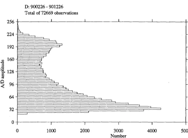
Three main appendices provide a reference manual for the computer soft-ware associated with the AMOR project. These are all written in Turbo Pas-cal 5.0. Appendix A gives brief descriptions for about 120 programs devel-oped on the PC during the last two years and considered important for a maintenance and development base for AMOR. Turbo Pascal uses a system of code modules to break software up into manageable files. Descriptions of the routines available within these subroutine library units are contained in Appendix B. Listings of the computer code directly involved in servicing the radar during an observing run and subsequent data reduction are included in Appendix C. A final Appendix D showing the overall distributions of mea-sured station data and orbital elements is included. This includes data for the approximately 1.32 X 105 _{meteor orbit observations made in the 14 months}

(29)

Chapter

2

Radar Hardware

The physical components of the AMOR system are described in this chapter. Successful operation of the radar requires the reliable simultaneous functioning of all these components. The process of achieving this was a substantial part of my thesis work. Individual components were made more reliable or modified to work as required. Occasionally this involved redesign or even complete abandonment of the component. All the components described here, except the transmitter, have been modified, built or rebuilt at least once as part of my research work. The hardware falls into several groups each discussed in a separate section.

2.1 Radio Frequency Components 14

Transmitter, AM Receivers, Phase Comparison.

2.2 Aerials 2:3

Collinear Receiver Arrays, Rhombic Transmitter Array.

2.3 AMOR Limiting Magnitude 37

2.4 FM Data Links 38

2.5 Digital hardware 42

A/D conversion, Timing Control, DMA Interface, DMA Controller.

2.6 Decommissioned Equipment 46

The computer is a IBivi-compatible MAC AT. The system was assembled in a 'Luggable' case rather reminiscent of a 'portable' sewing machine. It has 640 kBytes of directly accessible memory and a 385 kByte extended memory. The computer operates on a 12 MHz clock cycle1 . A 40 MByte hard disk drive is installed for data storage and program development. Software packages and

1_It

was found necessary to upgrade the RAM from 120 ns to 100 ns chips to make this possible. The observing software was developed to operate at the 12 MHz speed. In trying

(30)

utilities are kept to a minimum. An Ethernet card provides communication facilities to the rest of the world.

In the spirit of a first year laboratory report I have made a list of the major components to give a feel for the complexity of the system and the sheer logistical exercise of getting it all working:

Transmitter 1

A/D Conversion channels 5

Transmitter Array 1

Receiver Aerial Arrays 4 Timing Control Board 1

DMA Interface Card 1

26.2 MHz AM Receivers 4

Luggable AT Computer 1

RX Phase Comparator 1

\TAX Nlainframe 1

FM Link Transmitters 2

Magnetic Tape Drive 1

FM Receivers 2

2.1

Radio Frequency Components

The AMOR system detects meteors using a radar operating on 26.2 MHz. A trigger pulse is sent to the transmitter by the digital control board. The trans-mitter produces a 66 J.lS pulse. This is amplified to deliver a 7k\T, 70x40 rnA

pulse to the transmitter aerial array. The returning echo is collected by the receiver arrays. The subsequent passage of the signal through to the A/D converters is outlined in Figure 2.1. At the remote sites the video signal is fed directly into the FM link transmitter. At the Home site the FM link receivers demodulate the signal and send the amplitude information to the A/D con-verters. The signal from the south and north Home site aerials are each fed into a 26.2 MHz receiver. The video signal from the south receiver gives the Home site echo amplitudes. The local oscillator in the north receiver provides a reference for the phase linked south receiver. The video outputs from the two linked Home site receivers are fed into the phase comparison hardware. This produces a linearised sine and cosine amplitude output that is converted to a digital signal.

2.1.1 Transmitter

The 26.2 MHz transmitter was built in 1969. Since then it has had a long history of service. The transmitter was designed for an average power input of 1 kW. A maximum average power output of around 700 Watts could be expected. The transmitter is run at 7 k\T and 70 mA. This gives an average power output of 490 Watts. Running the transmitter well under full power provides a considerable enhancement in reliability. Doubling the power would

(31)

2.1. RADIO FREQUENCY COMPONENTS

..

..,

= ~ :a

~

tc

!;-" !;-" _~ ;; <Q 1l

" ll'!

s:

"

"'

...

u

~

~ l -;: ;

~J

I .,

l3 _!l"' ₀ _"' "'

~J

:l:!.~j6j :l:!.ljc;; ::;: .,g" ::;: '€ 0

<"'l " s <"'l 0 ~ <"'l 'ii _{<"'l ·"'}

C'l _r~>:C0 0 _C'lz::: _C'lz _C'l~

Figure 2.1: The radio frequency layout. of the AMOR system. The schematic shows the data flow from the 26.2 MHz aerials through to the

A/D converters and digital data logging system.

[image:31.599.176.468.139.692.2]

(32)

only give a

V2

improvement in the echo strength. The extra labour involved in maintaining this is not justified.2

With its advanced age the number of component failures in the transmitter has increased. It seems that power surges through the mains produce a fair number of these. A combination line filter and power regulator was added, substantially reducing the number of failures. This unit was contained in an orange box. The advantageous seemed to be confirmed with the increased failure rate when the original orange box was stolen after several months of trouble free operation. The meteor transmitter shares the transmitter hall with a 2.4 MHz transmitter used to measure mesospheric winds by partial reflection drifts. The concurrent operation of these transmitters produces a heavy load with considerable voltage drop on the mains transmission to the building. The presence of the mains regulator helps to keep the power of the the meteor transmitter up.

The radar pulses should be longer than the microsecond that it takes the transmitter output to rise from zero to peak power. With increased pulse length the range resolution deteriorates. The transmitter produces a relatively long 66 ps pulse to get power into a narrow bandwidth.

A trigger pulse is sent to the transmitter every 2.64 ms. This produces a pulse rate of 379 Hz. This pulse rate combined with the pulse duration produces a duty cycle of 40:1. The 490 W average power is concentrated into 20 kW pulses. Within the limits of average power noted above the transmitter could be used at any pulse rate. Originally the power supply of the transmit-ter was composed of three lpF capacitors. The continuous operation of the transmitter at this high pulse rate increased the duty cycle on these capaci-tors. The dielectric started to melt and ooze out the top of them. They were replaced in 1988 with two more modern 2 pF capacitors half the physical size of each of the originals. The power supply is capable of producing 1.6 kW DC power.

The trigger pulse is amplified through four stages and used to trigger the Driver. The final amplification is done by four Cll49 /1 tetrodes in the Power Amplifier3 • _{An adjustable inductive coupling connects the final stage to the} TX transmission line. 4

2_{The time lost whilst the transmitter is repaired reduces the number of meteor orbits}

ob-tained. This would probably eliminate the increase in orbit observations gained by increasing the power.

3_{Having done some research work on lung physiology I always thought the PA was some}

oblique reference to the Pulmonary Artery.

4

When I originally met the transmitter I thought of it as a large black box that produced 66 f.lS radio pulses at the prescribed rate. This acquaintance has now been refined to a stack

(33)

2.1. RADIO FREQUENCY COMPONENTS 17

2.1.2 Receivers

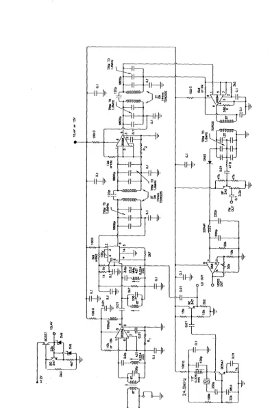
The AMOR system contains four 26.2 MHz receivers. A circuit diagram de-scribing the electronic layout of them is found in Figure 2.2. The receivers have an input impedance of

son.

A tuned circuit and amplification stage pre-cede the mixer in the receiver. A 24.6 MHz crystal provides the local oscillator reference. Two 23.0 MHz traps are included to filter out the IF image. Three stages tuned to the 1.6 MHz intermediate frequency amplify the signal on the IF strip. Finally the video receiver output is generated. This ranges from 0 to 10 volts. The signal is taken along the backplane of the receiver rack and then through a coaxial cable to the A/D converters. The noise at the output of the receivers, without a 50

n

load attached, is equivalent to 0.2 flY at the input.

The individual receiver bandpass characteristics and amplitude calibration curves are discussed below. In general they have a 20 kHz bandpass. Within the receiver power range the video output is reasonably linear. For the Home site receivers this corresponds to a signal strength ranging from 2 to 35 f.LV. The video output on the remote site 26.2 MHz receivers is set low to ensure the modulated FM signal of the links stay within their frequency range. The final video voltage to the A/D converters for the remote site channels is controlled in the FM link receivers. The calibration curves for the remote site channels show the amplitude response after transmission through the FM links.

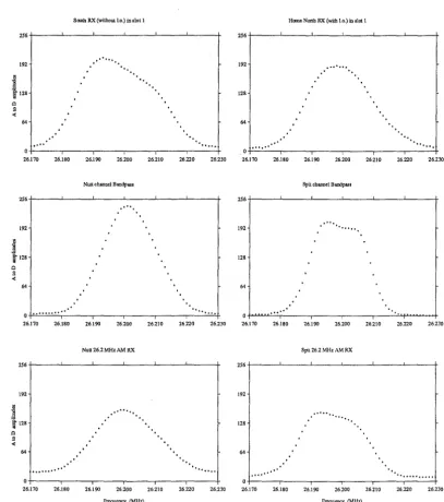
Receiver Bandpass

The receiver bandpass diagrams for each of the 26.2 MHz receivers are shown in Figure 2.3. The bandpass curves of the remote site channels as output by the FM link receivers are also plotted. A Marconi 2019A digital signal generator was used to measure these curves. Using a constant input signal strength the generator was scanned through the frequency range in 1 kHz steps. The video level for each point was measured using the A/D converters and then recorded by the computer. The data can be collected with the Ba.ndRX.Pas program and displayed with BandDraw.Pas.

The receivers were designed to have a 3 dB bandwidth of 20 kHz. The measured bandwidths range from 20 to 25 kHz (as may be seen in Figure 2.3) and the response curves reasonably symmetric about 26.2 MHz. The com-bination of the Home site receiver without the local oscillator and the south aerial seemed to be least susceptible to interference from external sources.

(34)

a

~ ~

ii

:;: N

:r _jl•

:::!:

rl''-1'·

(0

..f

N

~

[image:34.604.59.457.108.703.2]

(35)

2.1. RADIO FREQUENCY COMPONENTS

South RX (without to.) in slot 1 H001c Nonh RX (with l.o.) in .sht 1

256 256

···

192 192

···

'•

n

'•

J

128 128

"'

s

<

64 64

....

···

...

26.170 26.180 26.190 26200 26210 26220 26230 26.170 26.180 26.190 26.200 26.210

Nuttcbanocl Bandpass Spit cb&nncl Bandpa.u

256 256

192 192

···

n

~

~ 128 128

"' g

<

64 64

···

....

.

....

26.170 26.180 26.190 26200 26210 26220 26230 26.170 26.180 26.190 26200 26210

Nutt 26.2 MHz AM RX Spit 262 MHz AM: RX

256 256

192 192

n

~

....

,

... ....

~ 128 128

"'

s

<

64 64

···

...

....

···

.

..

26.170 26.180 26.190 26200 26.210 26220 26230 26.170 26.180 26.190 26200 26.210

rnquency (MHz) Frequency (MHz)

Figure 2.3: The bandpass response curves for the receivers. The curves were measured 1989 August 8. The frequency was shifted in 1 kHz steps, the video output measured through the A/D converters and recorded by the computer. The top four panels measure the receiver channels as they would appear at the Home site computer interface. The N utt and Spit. channel bandpass plots include transmission of the data through the FM links. Band-pass curves for t.he two remote site 26.2 MHz AM receivers are included for comparison.

19

···

26220 26230

26.220 26230

···

[image:35.600.94.502.166.627.2]

(36)

in trying to improve both the shape and position of the receiver bandpass responses. The values of the trimming capacitors in the three stages on the IF strips were adjusted to improve the response. The result is a compromise between the narrowest possible bandpass, its symmetry and the proximity to 26.2 MHz. It was found the shape varied noticeably over the hour after the receiver was turned on complicating the adjustment5

• A final trimming was

left until the receiver had been running continuously for a hour.

Receiver Calibration

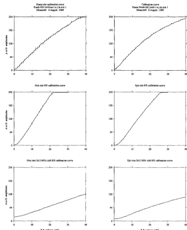
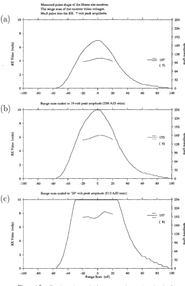
The receivers were calibrated using the Marconi signal generator mentioned above. The radio frequency signal strength was increased from 1 1.1.V in 1 f.J.V

steps until the individual receiver channel was saturated. The results of this calibration are shown in Figure 2.4. The calibration curves for the video output of the 26.2 MHz receivers located at the remote sites are included for reference.

The FM data link introduces uncertainties in the amplitude of the remote site echo profiles. These are discussed in more detail in the chapter on data reduction. Figure 2.4 clearly shows the two gain settings of the remote site video outputs; once at the AM receivers and again at the FM link receiver. The Home site South receiver channel was chosen to give the reference amplitude for all meteor echoes detected. The calibration curve for this receiver is shown on an enlarged scale in Figure 2.5.

It should be mentioned here that the echo amplitudes recorded in the observation records are not direct measurements of the echo amplitude at that range bin. The rangebin sample could be at any position with respect to the peak echo amplitude. A quarter, half, quarter average on adjacent rangebins is recorded as the profile amplitude for that sweep. This recorded A/D amplitude is not the peak strength of the echo. It cannot be directly applied to the calibration curves in this section to give the radio frequency signal strength of the echo. Section 4.2.3 discusses the relation of recorded amplitude to peak echo amplitude.

Home Site Phase Comparison

The relative phase angle of the echo on each of the two Home site aerials needs to be measured. The two Home site receivers use a common local oscillator mounted in the North receiver. The two 1.6 MHz I.F. signals are used to make a phase comparison between them. This comparison is done by a third units mounted in the receiver rack. Each signal is fed into a phase locked oscillator which generates an essentially square pulse related to the phase of the signal.

5_If_{memory serves me correctly there was some variation with signal amplitude to be}

(37)

2.1. RADIO FREQUENCY COMPONENTS

256

192

j

~ 128 0 ~ 64 0 0 256 192 .g ~ i 128 0 g < 64 0 0 256 192 .g

i

128 0

g

<

64

Hcme site calibration curve Calibrat.ioo curve

South RX (without l.o.) in slot 1 Heme North RX (wilh l.o.) in .slot 1

Mca&Urcd 6 August 1989 Meastmd 6 August 1989

256

192

128

64

10 20 30 40 10 20 30

NLttt site RX calibralion curve Spit &itc RX callbralioo curve

256

192

128

64

0

10 20 30 40 0 10 20 JO

Nutt site 26.2 MHz AM RX calibratioo curve Spit site 26.2 MHz AM RX calibratioo curve

256

192

128

64

10 20 30 40 10 20 30

R.F. volta.gc (uV) R.F. voltage (uV)

Figure 2.4: The calibration curves for the three receiver channels. The input signal strength is plotted against A/D amplitude of the video output voltage. The error bars plot the standard deviation of a series of samples taken on the stated signal strength. The calibration curves were measured on 1989 August. 6.

21

40

[image:37.599.107.481.186.646.2]

(38)

,g

.§

192

f

128

0

s

<t:

64

Home site calibration curve South RX (without l.o.) in slot 1

Measured 6 August 1989

0~---.---r---.---+

0 10 20 30 40

R.F. voltage (uV)

[image:38.598.116.440.281.590.2]

(39)

2.2. AERIALS 23

Radio noise will lock the circuit but produce random results for the phase difference between the two input signals. A echo with reasonable amplitude will cause the loop to lock at the phase of the input signal.

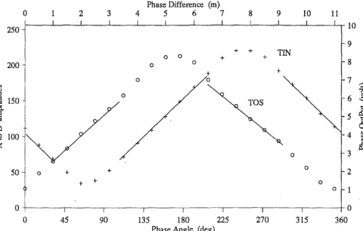
The two signals are fed into phase sensitive detectors, the output of which will be related to the differential phase. Combining square pulses will produce a triangular output. One signal is shifted by 90° for the second detector to provide enough information to determine the quadrant of the phase. The calibration of these Tin and Tos voltage outputs are discussed in Section 4.3.1.

2.2

Aerials

The AMOR system includes a total of nine aerials. Four collinear receiver arrays and one rhombic transmitter array are designed to operate at the radar frequency of 26.2 MHz. The remaining four are the three element Yagi aerials of the two 39 MHz FM data links. The aerials have a broad enough band so that small changes in the operating frequency can be handled. for example from 26.36 to 26.2 MHz and from 39.6 to 39.0 MHz.

The original design of the system meshed the transmitter and receiver patterns together. The two aerials were arranged so that the first null of the transmitter pattern fell at the same point as the secondary maximum of the receiver arrays. This produced the narrowest effective beam with the shortest possible aerials. In retrospect the narrow beam should have been achieved using the transmitter array only. This would have reduced the labour in developing and maintaining four long receiver aerials. Broader arrays would ensure that all three receiver sites have the greatest likelihood of detecting an echo from any illuminated meteor trail.

The transmitter aerial produces a narrow beam in azimuth but with a broad distribution of power in elevation. Matching loads at the ends of the rhombics phased the array so most of the power was directed south. The position of the meteor trail could be assumed without too much danger of ambiguity6_. _{The collinear receiver aerials give a narrow beam to both the} north and south. In fact the timelags determined from echo amplitude profiles can unambiguously place the trails in either the north or south lobes. A new collinear transmitter array has been built and awaits commissioning. This will radiate equally both north and south. The detection of particles from polar orbits will be improved. This new array is considerably longer than the current transmitter aerial. A narrower beam with greater peak field intensity will be achieved. This should move the detection limit to a fainter magnitude. The accuracy in angular position of the meteor will be improved.

6

(40)

1984 August 24-A coax array fed at six locations. Coax cable provided the active elements with the core and shields swapped every half wavelength.

1986 January Open wire 24.A collinear aerial with two feed points.

1986 November Remote site aerial relocated from the Swamp to Nutt site. 4A single feed open wire collinear.

1988 November Nutt site extended to 12-A with one feed point.

1989 February Transmission line added and Nutt site brought in line with other 24A aerials.

1989 August After measuring the power diagram associated with this con-figuration the receiver aerials were changed to an array of 6 X 2.A bays. The two Home site aerials contained 8 bays.

1990 January The Spit site aerial was moved a further 4 km down the Kaitorete Spit.

Table 2.1: A short potted history of the collinear receiver arrays.

An estimate needs to be made of the measurement uncertainty in assum-ing the meteor detection points are on the meridian. Both the orientation and width of the beam determine this. Beam width contributes the biggest uncer-tainty. Crudely, the location is known to within the 3 dB half power points of the aerial array power distribution patterns. The radar magnitude of meteor echoes detected by the system depends on the gain of the aerial arrays. This gain is the ratio of the peak power radiated by the antenna. to a theoretical equidirectiona.l power distribution.

2.2.1 Collinear Receiver Arrays

The 26.2 MHz receiver aerials are composed of centra.lly fed 2.A collinear sec-tions in a. broadside array. The field station at Birdlings Flat is an extremely corrosive sea-side environment It is exposed to both southerly storm fronts and nor-west gales. Considerable work was done to make these receiver arrays reliable under these conditions. Table 2.1 gives a brief history of the receiver aerials.

(41)

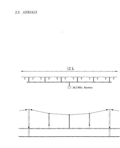
2.2. AERIALS

12

A.

_....

--

...

--I

I

Figure 2.6: A schematic diagram of the collinear receiver array. The top sketch shows an elevation of the N utt site aerial layout as it finally evolved. A detail of one collinear bay is drawn at the bottom. Insulator connectors are shown as filled symbols. Two

twin coaxial cables join the aerial to the main transmi~sion line.

The matching stubs are secured to spacer rings in the t.ransmis-sion line with rope.

[image:41.600.71.480.66.567.2]

(42)

receiver bays is included in Figure 2.6. The solid rectangles represent perspe

A meteor orbit radar

METEOR ORBIT RADAR

SUBMITTED IN PARTIAL FULFILMENT OF THE REQUIREMENTS FOR THE DEGREE

Andrew D. Taylor

LIBRARY THESIS

Abstract

Contents

1 Introduction

2 Radar Hardware

4 Radar Data Reduction 73

5 Fresnel Velocity Measurements 145

Acknowledgements

B Unit File Descriptions 313

List of Tables

List of Figures

LIST OF FIGURES

Chapter

Visual Meteor Observations

1.2.1 Visual Orbit Determinations

1.2.2 Photography

1.2.3 TV Cameras

Radar Orbit Measurement Techniques

1.3.1 Range-Time

1.3.3 Continuous Wave Technique

Review of Previous Orbit Radars

1.4. REVIEW OF PREVIOUS ORBIT RADARS 7

Christchurch Meteor Orbit Radar

AMOR Thesis Layout

1.6. AMOR THESIS LAYOUT 11

Chapter

Radio Frequency Components

2.1.1 Transmitter

2.1. RADIO FREQUENCY COMPONENTS 17

Receiver Bandpass

2.1. RADIO FREQUENCY COMPONENTS

Receiver Calibration

Home Site Phase Comparison

Hcme site calibration curve Calibrat.ioo curve

2.2. AERIALS 23

Aerials

2.2.1 Collinear Receiver Arrays