Generating Virtual Even Aged Silver Fir Stand Structure Based on the Measured Sample Plots

Generating Virtual Even-Aged Silver Fir Stand Structure

Based on the Measured Sample Plots

OriGinAl SciEntiFic PAPEr

Karlo Beljan

_{, Mislav Vedriš}

_{, Stjepan Mikac}

_{, Krunoslav teslak}

DOI: https://doi.org/10.15177/seefor.16-16

(1) University of Zagreb, Faculty of Forestry, Department of Forest Inventory and Management, Svetošimunska 25, HR-10000 Zagreb, Croatia; (2) University of Zagreb, Faculty of Forestry, Department of Forest Ecology and Silviculture, Svetošimunska 25, HR-10000 Zagreb, Croatia

* correspondence: e-mail: kbeljan@sumfak.hr

intrODUctiOn

Prior to planning forest management, field measure-ments have to be done in order to obtain main forest characteristics. Because of its complexity and labour cost, field measurements are usually carried out on a previously chosen sample area, and not in the entire forest area [1-3]. This assumes that the unmeasured parts of the stand have the same or similar characteristics as the measured parts with the given confidence interval. The sample usually consists of many relatively small and spatially separated areas (e.g. 500 m2 _{in size) in order to estimate the variability} in statistical analysis, but it does not enable insight into the entire stand. By compilation of spatially separated plots into a single coherent plot, forest stand can be shown in its absolute area [4-7] and as such it can be used in forest tree growth simulators [8] for the purpose of planning

future forest management [4, 9-12]. Also, the compilation of spatially separated plots into a single coherent plot reduces the costs of the total measurement of structural elements of the entire stand [9]. Apart from the possibility of using virtual stands as a starting point for future forest management simulation, they can also be used for comparison between the present and the future value of forest resources [13].

Trees which belong to a stand can be classified according to their mutual position into three basic spatial patterns: i) clustered, ii) random, iii) regular [14]. This classification treats forest as two-dimensional in its form, which differs from defining its structure as three-dimensional [11]. Pommerening [11] also stressed that most of the measures which describe the forest structure can be classified into two groups according to mathematical relations: ABStrAct

Background and Purpose: The aim of this article is to create a virtual forest stand based on the field measurement of spatially separated sample plots and to examine its credibility based on the deviation of the basic characteristics of the virtual stand as compared to the field measurements.

Material and Methods: Field measurements were made on 20 circular sample plots with a 20 m radius, set on a 100x100 m grid. By using the univariate Ripley’s K function the regularity of the spatial pattern of trees was analysed. The diameter distribution and the frequencies of height within individual diameter class were mathematically fitted and used for generating the virtual stand. The whole process of generating the virtual stand was done in the R software. Area of study are even-aged silver fir stands in the Croatian Dinarides.

results: The main unit of the virtual stand is a tree, with the purpose that the virtual stand can then be used as a basis for forest stand growth simulators. The result of the research was a virtual stand of 3 ha whose characteristics only slightly differed from the field measured plots. Within the virtual stand, special emphasis has been put on tree heights, which were generated according to the variability of tree height for trees of the same diameter at breast height.

conclusions: Considering the distribution of diameters at breast height, tree heights, the number of trees, basal area and volume, the virtual stand has minimal deviations from the situation in the field and it adequately shows variability measured in the field.

Keywords: virtual forest, forest planning, Ripley’s (K) analysis, distribution fitting, R software

citation: BELJAN K, VEDRIŠ M, MIKAC S, TESLAK K 2016 Generating Virtual Even-Aged Silver Fir Stand Structure Based on the Measured Sample Plots. South-east Eur for 7 (2): 119-127. DOI: https://doi. org/10.15177/seefor.16-16

distance-independent and distance-dependent. The spatial distribution of trees and their interrelationship based on tree species, diameter and similar factors, is primarily the result of the impact of habitat, but also of forest management. Stands consisting of several different tree species of different age and size are the most complicated for modelling [5, 11], unlike even-aged and pure stands.

Generating virtual forest stand is conditioned by the type of simulator which will simulate future theoretical and/ or practical management. According to Pretzsch et al. [15] and Ngo Bieng et al. [5], there are three levels of forest stand growth simulators (single-tree level, diameter class level and stand level). The classification is always conditioned by the basic input data [15], while it refers to the level of

simulation [16] . Simulators based on individual trees are the

most complex and they require detailed data about every single tree in the stand. It is especially important that the virtual stand of a single-tree level realistically represents the

measured stand [17] so that the results of the simulation of

management would be more realistic. When generating such a virtual stand, the spatial distribution of trees plays a crucial role. By directly joining separated spatial sample plots, the resulting spatial distribution of trees would not match the spatial distribution in the field because of the marginal trees of spatially adjoining plots. Therefore the spatial distribution of trees in a virtual stand has to include all the factors of spatial occurrence of trees in the field [8, 11, 17]. Virtual stand can cover a much larger area than the spatial sample based on which it was generated [4-6, 8], which is one of the reasons for creating a virtual stand in the first place. The aim of this article is to create a virtual forest stand based on the field measurement of spatially separated sample plots and to examine its credibility based on the deviation of the basic characteristics of the virtual stand as compared to the field measurements.

MAtEriAl AnD MEtHODS

Study Site and Data collection

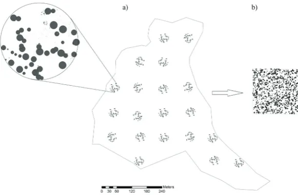
The study was conducted on an area of even-aged pure forests of silver fir (Abies alba Mill.) in Lika region, located in central Croatia (management unit Škamnica 44°58’N, 15°08’E). In forest of management unit Škamnica altitudes vary between 430 and 828 m a.s.l. Main soil types are limestone and dolomite. According to Köppen classification, the climate is marked as Cfwbx. Because of being even-aged and consisting of only one tree species (>95% of growing stock), this type of forest is rarely found in forest management of European fir forests [18]. Stands which belong to the observed forest are extremely similar to each other in terms of timber stock, stand basal area and increment [10]. The study site (management unit Škamnica) covers an area of 1833 ha, while the spatial sample obtained by field measurements is narrowed to a section (subcompartment) of 22.21 ha (Figure 1a).

Within a 100 m square grid oriented according to cardinal directions a total of 20 circular sample plots with 20 m radius were positioned. All trees within the plot (silver fir, beech (Fagus sylvatica L.) and other broadleaved

hardwoods (OBH)) with a diameter at breast height (dbh) over 10 cm were measured. For every tree, its species, the specific position in the three-dimensional space, dbh, and absolute height were determined according to the Croatian National Forest Inventory (CRONFI) field procedures [19]. Regarding the tree species and the status of the tree (dead/ alive) four subpopulations were determined: alive, fir-dead standing, beech, and broadleaved hardwoods. The total sampled area was 2.512 ha, which makes 11.3% of the studied stand’s area. Field measurements were conducted during 2013 after selective felling.

Spatial Structure Analyses

Ripley’s K(r) is a univariate function [20-22] used for the analysis of spatial structure. This function is based on the distance between all of the trees in a two-dimensional space [21], and it is often used in the analysis of spatial point patterns of forest ecosystems [23]. According to Ripley [20] and Ngo Bieng et al.[5], “Ripley’s K function is a function of the mean number of other trees found within distance r from a typical tree and it defines different degrees of random, clustered or regular spatial organisation”. In this study distance r around every tree is represented by a sequence of concentric circles with 0.5 m intervals. According to Besag and Diggle [24], L(r) square-root transformation of the main K(r) function was used.

The null hypothesis of the univariate function K(r) claims that there is no statistically significant difference between the spatial pattern of trees and the totally random spatial pattern, i.e. claiming that trees are randomly distributed. The confidence interval of totally random pattern was calculated by Monte Carlo simulation [25] with 99 repetitions of Poisson’s distribution [26]. The analysis was done with R software [27] using the “spatstat” package [28]. Generating Virtual Stand

Based on the analysis of spatial structure on all 20 plots a virtual stand was generated with a given condition that the spatial pattern of trees for all subpopulations is identical to the pattern in the field. The spatial pattern was generated with “stats” package, which is part of the R software [27]. The generated virtual stand is square-shaped and has an area of 3 ha (Figure 1b).

Furthermore, the virtual stand is assigned with additional conditions which describe positions measured in the field. The simulated positions of trees are associated with the corresponding subpopulation (tree species and the condition of being alive/dead), dbh and tree height. The association process consists of several parts:

i) The category of subpopulation (tree species and the condition of being alive/dead) has to be the same as in field measurements;

taken to be optimal, as according to Dziak et al. [34]. The fitting was done using the “fitdistrplus” package [35], which is a part of the R software [27]. The fitted distribution is associated with the allocation of the corresponding subpopulation in the area.

iii) The distribution of tree heights depending on dbh. The measured heights within a diameter class (5 cm) always include some variability. The measured heights were taken for every diameter class separately and their distributions within the class were mathematically fitted as described in ii). After this, the fitted distribution of heights was associated with the corresponding fitted dbh.

Virtual Stand Validation

Deviation of the measured characteristics of the virtual stand from the field measurements were analysed by diameter classes for every stand variable separately (the number of trees, basal area and volume). Also, two-sided K-S test [36, 37] was used for determining the statistically significant difference between them using the “stats” package [27], with significance level being 0.05. The test was conducted separately for each specific subpopulation (tree species, alive-dead) and in total for all the subpopulations together, i.e. for the entire stand.

rESUltS

Field measurements (Table 1) confirmed silver fir as the most frequent tree species in the study area. More than 80% of silver fir’s timber stock is concentrated in diameter class’s span between 37.5 cm and 62.5 cm, with diameter distribution characteristic for an even-aged stand (Figure 3a). Other subpopulations (dead standing fir trees, beech,

other broadleaved hardwoods) in timber stock are together represented by only 2.47% and on average do not achieve dbh greater than around 30 cm (Table 1).

The analysis of the spatial structure with the univariate Ripley’s K function was conducted for every sample plot separately (Figure 2). On a total of 19 plots, the spatial distribution of trees is random and it follows Poisson’s distribution while trees are grouped on one of the plots. The criterion of random spatial distribution of trees is reflected in the comparison of the transformed Ripley’s L(r) analysis for individual plots and Poissons’s random distribution (Figure 2). The result of clustered spatial patterns are groups of young trees (dbh=15-25 cm), which are situated on more open parts of the stand. From the results of the two-dimensional analysis it can be observed that the clustered pattern of trees is an exception, while random pattern prevails. Silver fir trees form the main stand (the upper storey), while other tree species can be found individually in the bush layer, i.e. in the lower storey.

According to the characteristics of the measured stand (Table 1), the number of trees in the virtual stand which were generated contained 375 trees∙ha-1_{, out of which 315} trees∙ha-1 _{were silver fir (alive), 43 trees∙ha}-1 _{were silver fir} (standing dead), 12 trees∙ha-1 _{were beech and 5 trees∙ha}-1 other broadleaved hardwoods. The spatial distribution of dbhs (Figure 1b) was generated based on the analysis of spatial patterns of individual subpopulations (Figure 2). The relative coordinates (x, y) within the stand were associated with the fitted diameter distribution (Figure 3). Although in some subpopulations the field measurements did not determine the presence of trees in every diameter class (Table 1), in the process of distribution fitting all classes were used for generating the virtual stand (Figure 3).

The coefficients of determination (r2_{) ranged from 0.70} to 0.85. The fitted distribution for the subpopulation of alive

3

2

1

0

-1

-2

-3

0 5 10 15 20

l

(r)

r (m)

silver fir had the highest coefficient of determination, which was 0.85. For the subpopulation of dead standing beech the coefficient was 0.79, for beech it was 0.70, and for other broadleaved hardwoods 0.82.

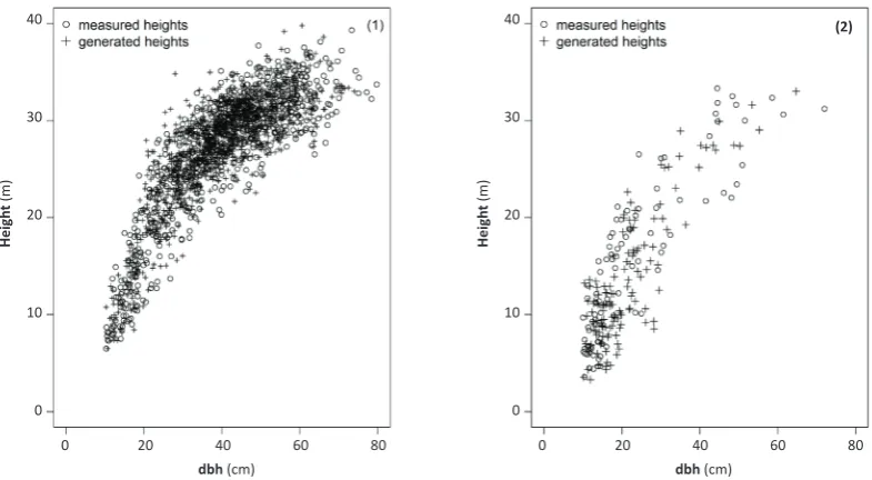
Tree height is a function of the tree’s dbh, which at this stage of generating virtual stand is already determined by its dimension and position. Figure 4 shows the comparison between the measured and the generated heights of alive and dead standing silver fir trees. Every diameter class was

associated with the number of tree heights proportional to the number of heights of that diameter class measured on the plots. Tree heights of beech and other broadleaved hardwoods were not generated by mathematical fitting because of the extremely small number of them (beech 12 trees∙ha-1_{, other broadleaved hardwoods 5 trees∙ha}-1_{), but} field measured heights were used instead.

The virtual stand generated this way includes the variability of the sampled actual stand. Mathematical

tABlE 1. Stand structure based on the measured field plots: stand density (N, trees∙ha-1_{), basal area (G, m}2_∙ha-1_{), volume (V, m}3_∙ha-1_).

FiGUrE 2. The results of univariate Ripley's (K) analysis for silver fir on all plots. Black lines represent the transformed values of Ripley's (K) analysis for the distance 0-20 m for each plot. The area of Poissons's random distribution with confidence interval of 95% is shown in grey.

* other broadleaved hardwoods dbh

(cm)

Abies alba Mill. Abies alba Mill. Fagus sylvatica l. OBH*

∑

Alive Dead standing Alive Alive

N

(trees∙ha-1_)(m2G_∙ha-1_)(m3_∙haV -1_)(trees∙haN -1_)(m2G_∙ha-1_)(m3_∙haV-1_)(trees∙haN -1_)(m2G_∙ha-1_)(m3V_∙ha-1_)(trees∙haN -1_)(m2G_∙ha-1_)(m3_∙haV -1_)(trees∙haN -1_)(m2G_∙ha-1_)(m3V_∙ha-1₎

12.5 13 0.16 0.89 20 0.24 0.95 7 0.08 0.43 2 0.02 0.15 41 0.51 2.42

17.5 22 0.54 4.19 11 0.27 1.55 2 0.05 0.38 35 0.85 6.12

22.5 20 0.83 8.83 6 0.24 1.85 1 0.03 0.21 2 0.07 0.62 29 1.16 11.51

27.5 27 1.62 19.36 3 0.19 1.12 1 0.05 0.71 31 1.86 21.19

32.5 33 2.78 35.62 1 0.09 1.00 1 0.04 0.37 36 2.91 36.99

37.5 44 4.91 67.49 1 0.05 0.63 45 4.96 68.13

42.5 45 6.26 89.64 1 0.06 0.90 1 0.10 1.44 46 6.42 91.98

47.5 47 8.38 122.93 1 0.07 1.09 48 8.45 124.02

52.5 31 6.65 99.44 1 0.08 1.18 32 6.73 100.63

57.5 20 5.19 78.51 20 5.19 78.51

62.5 9 2.67 40.01 9 2.67 40.01

67.5 2 0.85 12.97 2 0.85 12.97

72.5 1 0.15 2.28 1 0.15 2.28

77.5 1 0.37 5.66 1 0.37 5.66

fitting of diameter distribution and the distribution of tree heights resulted in particular deviations from the actual situation (Table 2). The comparison shown in Table 2 was done on the level of one hectare. The greatest deviations in distributions were recorded for alive silver fir trees (the

number of trees -5 trees∙ha-1_{, basal area 0.36 m}2_∙ha-1_{, and} volume 4.21 m3_∙ha-1_{). The results show that diameters at} breast height for silver fir of medium diameter classes (37.5-62.5 cm) have the greatest deviations, while for the lowest and highest diameter classes the deviations are significantly

FiGUrE 3. Diameter distributions for: alive silver fir (a), dead standing silver fir (b), beech (c), other broadleaved hardwoods (d); histograms represent sample plot data, line - mathematically fitted distribution.

FiGUrE 4. The comparison of measured and generated heights for alive (1) and dead silver fir trees (2). 10 20 30 40 50 60 70 80

10 20 30 40 50 60 70 80

10 20 30 40 50 60 70 80

10 20 30 40 50 60 70 80

n

(tr

ees∙ha

-1)

n

(tr

ees∙ha

-1)

N

(tr

ees∙ha

-1)

n

(tr

ees∙ha

-1)

dbh (cm)

dbh (cm)

dbh (cm)

dbh (cm) (a)

(c) (d)

(b) 50

40 30

20 10

0

8

6

4

2

0

8

6

4

2

0 50

40 30

20 10

0

0 20 40 60 80 0 20 40 60 80

dbh (cm) dbh (cm)

Heigh

t

(m)

Heigh

t

(m)

40

30

20

10

0

40

30

20

10

0

smaller. The difference of the virtual stand to the sample plots was calculated only up to those diameter classes for which the presence of trees was determined by field measurements.

In total, in the virtual stand the volume is greater only by 8.74 m3_∙ha-1_{, basal area is greater by 1.30 m}2_∙ha-1_{, and} the number of trees is smaller by 6 trees∙ha-1 _{(Table 2) as} compared to the results of field measurements (Table 1). The deviation for volume, shown in percentage (%), is 1.46%, for basal area it is 1.36% and for the total number of trees -1.06%.

Table 3 shows the results of the Kolmogorov-Smirnov test (K-S test) for the distributions of measured and generated values for dbh, tree height and volume of individual trees. With respect to the D value of the K-S test, deviations between the cumulative relative distributions of the two stands (measured and generated) are tested. The K-S test deviations for the subpopulation of beech were minimal, but the statistically significant difference between dbh and volume was recorded for the subpopulation of dead standing silver fir. According to this test, the subpopulation of alive fir does not have a statistically significant deviation from the situation in the field, which is especially important because this subpopulation makes 97% of growing stock and 84% of the number of trees in the stand. Also, in total (the comparison on the level of the entire stand) the difference is not significant.

DiScUSSiOn

Directly joining spatially adjacent plots into a single coherent plot would result in an incorrect spatial structure of trees in the areas where the adjacent plots are connected [11], but there is also a possibility of using such plots as a basis for forest stand growth simulators [38]. In the virtual stand the simulated spatial organisation (x, y) does not have identical distances between trees to those measured in the field, but the whole virtual stand meets the requirement of the spatial pattern (regular, clustered or random) with respect to the results of Ripley’s spatial analysis of individual subpopulations [5, 8-10]. Some authors [5, 6, 9, 11] agree with the claim that random distribution of trees is the most common and that generating a virtual stand according to random distribution is a less significant mistake. The only possible mistake caused by spatial pattern of trees might be found if the virtual stand is connected with forest stand growth simulators. In that case, the result of the stand’s future development can to some extent be influenced by the mutual position of subpopulations [9, 39, 40]. The disadvantage of the majority of virtual stands is not taking into account the three-dimensional aspect of the forest [41]. The analysis of spatial structure, as well as the generating of the relative coordinates (x, y), generally refers to the analysis of horizontal projections of trees’ positions. However, it is possible to generate relative coordinates of

tABlE 2. The deviation of the structural elements of the virtual stand from the plot data: stand density (N, trees∙ha-1_{), basal}

area (G, m2_∙ha-1_{), volume (V, m}3_∙ha-1_).

dbh (cm)

Abies alba Mill. Abies alba Mill. Fagus sylvatica l. OBH*

∑

Alive Dead standing Alive Alive

N

(trees∙ha-1_)(m2G_∙ha-1_)(m3_∙haV -1_)(trees∙haN -1_)(m2G_∙ha-1_)(m3_∙haV-1_)(trees∙haN -1_)(m2G_∙ha-1_)(m3V_∙ha-1_)(trees∙haN -1_)(m2G_∙ha-1_)(m3_∙haV -1_)(trees∙haN -1_)(m2G_∙ha-1_)(m3V_∙ha-1₎

12.5 -5 0.00 -0.11 -8 0.00 -0.30 0 0.00 0.00 0 0.00 0.00 -13 0.00 -0.41 17.5 -9 0.00 -1.29 5 0.00 1.67 0 0.00 0.00 0 0.00 0.00 -4 0.00 0.38 22.5 -1 0.00 -0.03 4 0.00 1.76 0 0.00 0.00 0 0.00 0.00 3 0.00 1.73

27.5 8 0.40 5.54 1 0.00 1.17 0 0.00 0.00 0 0.00 0.00 9 0.40 6.71

32.5 1 0.10 0.99 1 0.00 1.55 -1 0.00 -0.10 0 0.00 0.00 1 0.10 2.44

37.5 6 0.70 9.81 1 0.00 0.32 0 0.00 0.00 0 0.00 0.00 7 0.70 10.13

42.5 6 0.90 11.60 -1 0.00 -0.10 -1 0.00 -0.20 0 0.00 0.00 4 0.90 11.30

47.5 -10 -2.00 -27.60 0 0.00 0.00 0 0.00 0.00 -10 -2.00 -27.60

52.5 -6 -1.00 -22.90 -1 0.00 -1.20 -7 -1.00 -24.10

57.5 1 0.30 5.20 1 0.30 5.20

62.5 1 0.40 5.64 1 0.40 5.64

67.5 1 0.30 4.98 1 0.30 4.98

72.5 2 1.20 18.00 2 1.20 18.00

77.5 -1 0.00 -5.66 -1 0.00 -5.66

K-S test

Abies alba Mill. Abies alba Mill. Fagus sylvatica l.

∑

Alive Dead standing Alive

dbh Height Volume dbh Height Volume dbh Height Volume dbh Height Volume

N1/N2* 800/933 75/135 30/33 915/1111

D 0.054 0.061 0.061 0.290 0.102 0.216 0.069 0.042 0.072 0.043 0.035 0.040

p value 0.1585 0.0763 0.0792 0.0005 0.4911 0.0219 1.0000 1.0000 1.0000 0.2950 0.5434 0.3679 * the ratio between the number of measured and the total number of generated trees

D – maximum difference of cumulative values

trees by using digital terrain model (DTM), but the horizontal projections would be identical. This is also corroborated by the characteristics of forest stand growth simulators which mostly work with horizontal surfaces [15]. The object of this research is characterised by up to 10% of inclination which could be ignored without having any significant mistakes as a consequence in further simulations of this stand’s management.

In this research, the analysis of spatial distribution was done with the univariate Ripley’s function for every individual subpopulation. Even though the subpopulation of silver fir (alive) holds more than 97% of timber stock, the bivariate analysis was not done because the contribution of other subpopulations was too small. In case there are more subpopulations and all of them are represented by 10% or more, it is possible to conduct an adequate bivariate analysis for all populations, as it was done by Pretzsch [8], Goreaud et al. [42] and Grabarnik and Särkkä [43]. In other words, in this paper the subpopulations were analysed independently of each other because only one subpopulation was dominant. In case of an even-aged pure stand of silver fir, the assumption taken was that there was no significant spatial interaction between the subpopulations.

Tree height is a function of its diameter at breast height and it is natural that trees of the same diameters at breast height are of different heights [44-47]. In this study tree heights were not associated with their corresponding diameter based on height–daimeter equations (e.g. by using Michailoff’s function [48]), beacuse the fitted height curve does not describe variability within the same diameter class and thus reduces the variability of heights of real forest stand. Therefore in this study the variability of heights was associated with the corresponding diameter at breast height in a way that the distribution of heights within the same diameter class were taken into account (Figure 4). The presented way of generating virtual stand in this segment differs from the majority of similar studies.

When simulating a virtual stand it is fully expected that some deviations from field measurements will occur (Table 2). The comparison presented in Table 2 has been done on the area of one hectare, which is an adequate measure for this purpose. The virtual stand was generated based on a methodology which will always, on average, result in the

same characteristics, no matter the size of the area. The Kolmogorov-Smirnov test was done for all measured trees in the field (2.512 ha) and all trees belonging to the 3 ha area of the virtual stand. The deviations were primarily a result of the mathematical fitting of diameter distribution and the variability of tree heights within the same diameter class. Although the best possible fitting functions were used, they are still equations, and therefore they cannot completely stochastically describe all the variability in a forest stand [29]. In Figure 3 it can be seen that particular subpopulations are not continuously represented in all diameter classes, but appear intermittently in fitted distribution. In such cases, due to using continuous mathematical functions, the result of fitting always has to be greater than zero (Figure 3). There are no deviations for the subpopulation of other broadleaved hardwoods because the dimensions are identical to those measured in the field, so neither the K-S test is shown in Table 3. The distributions for this subpopulation are identical in the measured and in the virtual forest because of a very low frequency of only five trees per hectare, which was easier to generate.

The final result of this study is a virtual stand of 3 ha. According to Čavlović et al. [49], and Čavlović and Božić [50], that is the minimal area on which it is possible to establish a selective structure in the range of beech-fir forests of the Croatian Dinarides. On the other hand, the minimal stand area for sustainable even-aged forest management is one hectare. Therefore this generated area of the virtual stand is at the same time the universal and the minimal area for further management simulation in its two basic forms: the selective and the regular form. This is corroborated by the fact that silver fir supports both forms of management [10]. For the aforementioned management simulation, the virtual stand should be connected to one of the forest stand growth simulators on the level of one tree. Although this is a virtual stand in which for every tree many characteristics are known (position, species, diameter, height), the projection of future management which involves felling on the level of a single tree would be made difficult and very impractical for a virtual stand with a larger area (e.g. 10 ha, 20 ha or 50 ha). An area of 3 ha enables the user to decide in a relatively short period of time which tree should be cut, but that the result of management simulation is the same as the result

from a much larger area.

Before generating a virtual stand, data have to be collected by field measurement. Forest management and inventory is prescribed by the regulations of a particular country. In intensive standwise inventories forest stands are measured cyclically every ten years in order to develop management plans. However, those data are still not enough for generating a virtual stand. What is missing are the data about the spatial pattern of trees. This kind of research leads to the possibility of updating the abovementioned data with the spatial structure which can be determined in a relatively short time and at low cost. Stands are already organised based on the structural similarities within them so it is expected that the spatial pattern and analysis within them would be the same. This way it is possible to create entire virtual forests [16].

cOnclUSiOn

Considering the distribution of diameters at breast height, tree heights, the number of trees, basal area and volume, the virtual stand has minimal deviations from the situation in the field and it adequately shows variability measured in the field. Variability is an inherent component

of the most common stand characteristics which has to be determined when planning and managing forests. It is obvious that the characteristics of ground vegetation, shrubs, ground water and the like would not match the situation in the field. However, the presented methodology can have its role in ecology and can upgrade the process of generating virtual stands.

The virtual stand generated as part of this research can be used as a basis for forest stand growth simulators whose basic unit is a single tree and this way it can examine various future scenarios for managing both forest stands and entire forests. In that case, a virtual stand has to be generated for every part of the area managed as a separate stand (sub-compartment), because the virtual stand represents only a single stand within the entire forest. Virtual stands can be used in several different branches of forestry for which the size of the area is the most important factor, for example in landscape management. As part of a long-term forest management planning, generating virtual stands and using them in forest stand growth simulators should become a standardized procedure with the aim of predicting future forest characteristics as realistically as possible. The logical continuation of such plans is using forestry economics in order to provide an answer to the question of which potential future scenarios are economically justifiable.

rEFErEncES

1. JAZBEC A, VEDRIŠ M, BOŽIĆ M, GORŠIĆ E 2011 Efficiency of inventory in uneven-aged forests on sample plots with different radii. Croat J For Eng 32 (1): 301-312

2. VEDRIŠ M, JAZBEC A, FRNTIĆ M, BOŽIĆ M, GORŠIĆ E 2009 Precision of structure elements’ estimation in a beech-fir stand depending on circular sample plot size. Sumar list 133

(7-8): 369-379

3. KANGAS A, MALTAMO M 2006 Forest Inventory: Methodology and Applications. Springer, Dordrecht, The Netherlands, 362 p. DOI: https://doi.org/10.1007/1-4020-4381-3

4. HANEWINKEL M, PRETZSCH H 2000 Modelling the conversion from even-aged to uneven-aged stands of Norway spruce

(Picea abies L. Karst.) with a distance-dependent growth

simulator. Forest Ecol Manag 134 (1–3): 55-70. https://doi. org/10.1016/S0378-1127(99)00245-5

5. NGO BIENG M A, GINISTY C, GOREAUD F 2011 Point process models for mixed sessile forest stands. Ann For Sci 68 (2): 267-274. DOI: https://doi.org./10.1007/s13595-011-0033-y

6. NGO BIENG MA, GINISTY C, GOREAUD F, PEROT T 2006 First typology of oak and scots pine mixed stands in Orléans forest (France), based on the canopy spatial structure. New Zeal J

For Sci 36 (2/3): 325-346.

7. DEGENHARDT A, POMMERENING A 1999 Simulative Erzeugung von Bestandesstrukturen auf der Grundlage von Probekreisdaten. Sektion Forstliche Biometrie und Informatik im Deutschen Verband Forstlicher Forschungsanstalten, Volpriehausen, 15 p

8. PRETZSCH H 1997 Analysis and modeling of spatial stand structures. Methodological considerations based on mixed beech-larch stands in Lower Saxony. Forest Ecol Manag 97 (3): 237-253. https://doi.org/10.1016/S0378-1127(97)00069-8

9. STAMATELLOS G, PANOURGIAS G 2005 Simulating spatial distributions of forest trees by using data from fixed area plots. Forestry 78 (3): 305-312. DOI: https://doi.org/10.1093/ forestry/cpi028

10. BELJAN K 2015 Economic analysis of even-aged silver fir

(Abies alba Mill.) forest management. PhD thesis, University

of Zagreb, Croatia, Zagreb, 166 p

11. POMMERENING A 2002 Approaches to quantifying forest structures. Forestry 75 (3): 305-324. DOI: https://doi. org/10.1093/forestry/75.3.305

12. LAFOND V, LAGARRIGUES G, CORDONNIER T, COURBAUD B 2013 Uneven-aged management options to promote forest resilience for climate change adaptation: effects of group selection and harvesting intensity. Ann For Sci 71 (2): 173-186. DOI: https://doi.org/10.1007/s13595-013-0291-y

13. BIGING G S, DOBBERTIN M 1995 Evaluation of Competition Indices in Individual Tree Growth Models. Forest Sci 41 (2): 360-377

14. DIGGLE P J 2003 Statistical analysis of spatial point patterns. Hodder Arnold, London, UK, 159 p

15. PRETZSCH H, BIBER P, DURSKY J, GADOW K, HASENAUER H, KÄNDLER G, GENK G, KUBLIN E, NAGEL J, PUKKALA T, SKOVSGAARD J P, SODTKE R, STERBA H 2002 Recommendations for standardized documentation and further development of forest growth. Forstwiss Centralbl 121 (3): 138-151. DOI: https://doi.org/10.1046/j.1439-0337.2002.00138.x

16. POTT M, FABRIKA M 2002 An information system for the evaluation and spatial analysis of forest inventory. Fosrtwiss Centralbl 121 (1): 80-88

18. KLOPCIC M, BONCINA A 2011 Stand dynamics of silver fir

(Abies alba Mill.)-European beech (Fagus sylvatica L.) forests

during the past century: a decline of silver fir? Forestry 84 (3): 259-271. DOI: https://doi.org/10.1093/forestry/cpr011

19. ČAVLOVIĆ J, BOŽIĆ M 2008 Nacionalna inventura šuma u Hrvatskoj - Metode terenskog prikupljanja podataka. University of Zagreb, Faculty of Forestry, Zagreb, Croatia, 146 p

20. RIPLEY BD 1976 The second-order analysis of stationary point processes. J Appl Probab 13 (2): 255-266. DOI: https:// doi.org/10.2307/3212829

21. RIPLEY BD 1981 Spatial Statistics. Wiley, New York, USA, 252 p

22. DIXON PM 2002 Ripley’s K function. In: Abdel HE (ed)

Encyclopedia of Environmetrics. Chichester, Wiley, pp 1796-1803

23. PERRY W GL, MILLER PB, ENRIGHT JN 2006 A comparison of methods for the statistical analysis of spatial point patterns in plant ecology. Plant Ecol 187 (1): 59-82. DOI: https://doi. org/10.1007/s11258-006-9133-4

24. BESAG J, DIGGLE P J 1977 Simple Monte Carlo tests for spatial pattern. Appl Statist 26 (3): 327-333. DOI: https://doi.

org/10.2307/2346974

25. WALLER LA, SMITH D, CHILDS JE, REAL LA 2003 Monte Carlo assessments of goodness-of-fit for ecological simulation models. Ecol Model 164 (1): 49-63. DOI: https://doi. org/10.1016/S0304-3800(03)00011-5

26. POISSON S 1837 Recherches sur la probabilité des jugements en matière criminelle et matière civile

27. R CORE TEAM 2015 R: A language and environment for statistical computing. R Foundation for Statistical Computing. Vienna, Austria. URL: https://www.R-project.org/ (15 June 2016)

28. BADDELEY A, RUBAK E, TURNER R 2015 Spatial Point Patterns: Methodology and Applications with R. Chapman and Hall/CRC Press, London, UK, 810 p

29. JAWORSKI A, PODLASKI R 2011 Modelling irregular and multimodal tree diameter distributions by finite mixture models: an approach to stand structure characterisation. J

For Res 17 (1): 79-88. DOI:

https://doi.org/10.1007/s10310-011-0254-9

30. BURKHART HE, TOMÉ M 2012 Diameter-Distribution Models for Even-Aged Stands. In: Burkhart HE, Tomé M (eds)

Modeling Forest Trees and Stands. Dordrecht, Heidelberg, London, New York, Springer, pp 261-309. DOI: https://doi.

org/10.1007/978-90-481-3170-9_12

31. GAUSS C F 1809 Theoria motus corporum coelestium in sectionibus conicis solem ambientium. Friedrich Perthes and I.H. Besser, Hamburg, Germany, 247 p

32. GALTON F 1889 Natural Inheritance. Macmillan & Co, London, UK, 259 p. URL: http://galton.org/books/natural-inheritance/pdf/galton-nat-inh-1up-clean.pdf (20 June 2016) 33. WEIBULL W 1951 A statistical distribution function of wide

applicability. J Appl Mech 18 (3): 293-297

34. DZIAK JJ, COFFMAN DL, LANZA TS, LI R 2012 Sensitivity and specificity of information criteria. College of Health and Human Development The Pennsylvania State University, Pennsylvania, USA, 30 p

35. DELIGNETTE-MULLER ML, DUTANG C 2015 fitdistrplus: An R Package for Fitting Distributions. J Stat Softw 64 (4): 1-34. DOI: https://doi.org/10.18637/jss.v064.i04

36. KOLMOGOROV A 1933 Sulla Determinazione Empirica di una Legge di Distributione. Giornale dell’Istituto Italiano degli

Attuari 4: 421-424

37. SMIRNOV N 1948 Table for estimating the goodness of fit of empirical distributions. Ann Math Stat 19 (2): 279-281. DOI:

https://doi.org/10.1214/aoms/1177730256

38. DVORAK L 2000 Kontrollstichproben im Plenterwald. PhD Thesis, ETH Zürich, Zürich, Switzerland, 176 p

39. HASENAUER H 2006 Sustainable forest management. Springer, Berlin, Germany, 398 p. DOI: https://doi. org/10.1007/3-540-31304-4

40. GOREAUD F, ALVAREZ I, COURBAUD B, DE COLIGNY F 2006 Long-Term Influence of the Spatial Structure of an Initial State on the Dynamics of a Forest Growth Model: A Simulation Study Using the Capsis Platform. Simulation 82 (7): DOI:

https://doi.org/475-495. 10.1177/0037549706070397

41. ZENNER EK, HIBBS DE 2000 A new method for modeling the heterogeneity of forest structure. Forest Ecol Manag 129 (1-3): 75-87. DOI: https://doi.org/10.1016/S0378-1127(99)00140-1

42. GOREAUD F, LOUSSIER B, NGO BIENG M A, ALLAIN R 2004Simulating realistic spatial structure for forest stands: a mimetic point process. Interdisciplinary Spatial Statistics Workshop, 22 p

43. GRABARNIK P, SÄRKKÄ A 2009 Modelling the spatial structure of forest stands by multivariate point processes with hierarchical interactions. Ecol Model 220 (9-10): 1232-1240. DOI: https://doi.org/10.1016/j.ecolmodel.2009.02.021

44. BARRIO ANTA M, DIEGUEZ ARANDA U, CASTEDO DORADO F, ÁLVAREZ GONZALES J, ROJO-ALBORECA A 2006 Mimicking natural variability in tree height of pine species using a stochastic height-diameter relationship. New Zeal J For Sci 36 (1): 21-34

45. CASTAÑO-SANTAMARÍA J, CRECENTE-CAMPO F, FERNÁNDEZ-MARTÍNEZ J L, BARRIO-ANTA M, OBESO J R 2013 Tree height prediction approaches for uneven-aged beech forests in northwestern Spain. Forest Ecol Manag 307 (0): 63-73. DOI:

https://doi.org/10.1016/j.foreco.2013.07.014

46. CASTEDO DORADO F, BARRIO ANTA M, PARRESOLC B, ÁLVAREZ GONZALES J 2005 A stochastic height-diameter model for maritime pine ecoregions in Galicia (northwestern Spain). Ann For Sci 62 (5): 455-465. DOI: https://doi. org/10.1051/forest:2005042

47. CASTEDO DORADO F, DIÉGUEZ-ARANDA U, BARRIO ANTA M, SÁNCHEZ RODRÍGUEZ M, VON GADOW K 2006 A generalized height–diameter model including random components for radiata pine plantations in northwestern Spain. Forest Ecol

Manag 229 (1-3): 202-213. DOI: https://doi.org/10.1016/j.

foreco.2006.04.028

48. MICHAILOFF I 1943 Zahlenmäßiges Verfahren für die Ausführung der Bestandeshöhenkurven. 6: 273-279 49. ČAVLOVIĆ J, BOŽIĆ M, BONČINA A 2006 Stand structure of

an uneven-aged fir–beech forest with an irregular diameter structure: modeling the development of the Belevine forest, Croatia. Eur J For Res 125 (4): 325-333. DOI: https://doi. org/10.1007/s10342-006-0120-z

50. ČAVLOVIĆ J, BOŽIĆ M 2007 The establishment and preservation of a balanced structure of beech-fir stands. Glas