Tübingen Oslo Team at the VarDial 2018 Evaluation Campaign: An Analysis of N gram Features in Language Variety Identification

55

T ¨ubingen-Oslo Team at the VarDial 2018 Evaluation Campaign:

An Analysis of N-gram Features in Language Variety Identification

C¸ a˘grı C¸ ¨oltekin♠ Taraka Rama♥ Verena Blaschke♠ ♠_{Department of Linguistics, University of T¨ubingen, Germany}

♥_{Department of Informatics, University of Oslo, Norway}

tarakark@ifi.uio.no, ccoltekin@sfs.uni-tuebingen.de, verena.blaschke@student.uni-tuebingen.de

Abstract

This paper describes our systems for the VarDial 2018 evaluation campaign. We participated in all language identification tasks, namely, Arabic dialect identification (ADI), German dialect identification (GDI), Discriminating between Dutch and Flemish in Subtitles (DFS), and Indo-Aryan Language Identification (ILI). In all of the tasks, we only used textual transcripts (not using audio features for ADI). We submitted system runs based on support vector machine classifiers (SVMs) with bag of character and word n-grams as features, and gated bidirectional recurrent neural networks (RNNs) using units of characters and words. Our SVM models outperformed our RNN models in all tasks, obtaining the first place on the DFS task, third place on the ADI task, and second place on others according to the official rankings. As well as describing the models we used in the shared task participation, we present an analysis of the n-gram features used by the SVM models in each task, and also report additional results (that were run after the official competition deadline) on the GDI surprise dialect track.

1 Introduction

Identifying the language of a text or speech is an important step for many (multi-lingual) natural lan-guage processing applications. At least for written text, the lanlan-guage identification is a ‘mostly-solved’ problem. High accuracy values can be obtained with relatively simple machine learning models. One challenging issue, however, is identifying closely related languages or dialects, which is an interesting research question as well as being relevant to practical NLP applications. The series of VarDial eval-uation campaigns (Malmasi et al., 2016; Zampieri et al., 2017; Zampieri et al., 2018) included tasks of identifying closely related languages and dialects from written or spoken language data. This pa-per is a description of our efforts in the VarDial 2018 shared task, which featured four dialect/language identification tasks, as well as one morphosyntactic tagging task. We only participated in the language identification tasks.

The aim of the ADI task, which was also part of the earlier two VarDial evaluation campaigns, is to recognize the five varieties of Arabic (Egyptian, Gulf, Levantine, North-African, and Modern Standard Arabic) from spoken language samples. The task provides transcribed text as well as pre-extracted audio features and raw audio recordings. The DFS task, introduced this year, is on discriminating Dutch and Flemish subtitles. The GDI is another task that was present in earlier VarDial shared tasks, where the aim is to identify four Swiss German Dialects (Basel, Bern, Lucerne, Zurich). This year’s edition also included a surprise dialect. Finally, the ILI task, another newcomer, is about identifying five closely related Indo-Aryan languages (Hindi, Braj Bhasha, Awadhi, Bhojpuri, and Magah).

A simple approach to language/dialect identification is to treat it as a text (or document) classification task. Two well-known methods for solving this task are linear classifiers with bag-of-n-gram represen-tations, and, recently popularized, recurrent neural networks. As in our participation at earlier VarDial evaluation campaigns (C¸ ¨oltekin and Rama, 2016; C¸ ¨oltekin and Rama, 2017), we experiment with both

the methods. Although our main participation is based on the SVM models, we also report the perfor-mance of the RNN models for comparison, and provide further analyses regarding the feature sets used in the SVM models.

We outline our approach in the next section, describing the models used briefly and explaining the strategies we used for the GDI surprise dialect track. Section 3 introduces the data, explains the experi-mental procedure used, and presents the analyses and results from the experiments run during and after the shared task. After a general discussion in Section 4, Section 5 concludes with pointers to potential future improvements.

2 Approach

2.1 SVMs with bag-of-n-gram features

Our SVM model is practically the same as the one used in C¸ ¨oltekin and Rama (2016) and C¸ ¨oltekin and Rama (2017), which in turn was similar to Zampieri et al. (2014). Similar to last year’s participation, we used a combination of character and word n-grams as features.1 All features are concatenated as a single feature vector per text instance and weighted by sub-linear tf-idf scaling. For the multi-class classification tasks (all except the DFS task which is binary), we used one-vs-rest SVM classifiers. All SVM models were implemented with scikit-learn (Pedregosa et al., 2011) and trained and tested using the Liblinear backend (Fan et al., 2008).

2.2 Bidirectional gated RNNs

Our neural model, for this task, again based on our previous models (C¸ ¨oltekin and Rama, 2016; C¸ ¨oltekin and Rama, 2017), includes two bidirectional gated RNN components: one taking a sequence of words as input and another taking a sequence of characters as input. The recurrent components of the network build two representations for the text (one based on characters and the other based on words), the repre-sentations are concatenated and passed to a fully connected softmax layer that assigns a language label to the document based on the RNN representations. Both sequence representations are trained jointly within a single model. We experimented with two well-known gated recurrent network variants, GRU (Cho et al., 2014) and LSTM (Hochreiter and Schmidhuber, 1997). For both character and word inputs, we used embedding layers before the RNN layers. Character sequences longer than250characters and word sequences longer than100tokens are truncated. All neural network experiments were implemented with Tensorflow (Abadi et al., 2015) using the Keras API (Chollet and others, 2015).

2.3 GDI surprise dialect

After the submission deadline, we experimented with the surprise dialect track of the GDI task, wherein the test set contains the surprise dialect ‘XY’ in addition to the four dialects for which training and development sets had been provided. We used the tuned SVM model for the classification of the four known dialects, but changed its decision rule such that it allows the classifier to predict a fifth class as well. Our initial SVM system consists of one one-versus-rest (OvR) SVM classifier per dialect in the training data; and, the dialect predicted for a given sample is the one whose corresponding OvR classifier yields the highest decision function value for the sample.

We experimented with this decision rule by altering it in the following ways:

• Rejected by all: When a sample is rejected (i.e. classified as ‘rest’) by all OvR classifiers, it is predicted as XY.

• Accepted by several: When a sample is accepted by several OvR classifiers, it is predicted as XY.

• Rejected or multi-accepted: When either of the two previous rules applies, the label is predicted as XY.

• Standard deviation: The fifth of the test set where the OvR classifiers’ decision function values exhibit the smallest standard deviations is predicted as XY.

1_{‘Word’ refers to the strings produced by a simple regular-expression tokenizer that splits documents into consecutive}

• Difference: The fifth of the test set where the differences between the two highest decision function values are smallest is predicted as XY.

The last two rules na¨ıvely assume a balanced label distribution, which is actually not the case for the gold-standard test set. The four known dialects each constitute21–22% of the gold-standard labels whereas the surprise dialect only contributed14%.

3 Experiments and results

3.1 Data

The ILI and DFS tasks are new tasks that featured for the first time, whereas ADI and GDI are tasks that were present over the past years. The Arabic data set is based on Ali et al. (2016). This year’s shared task data included additional audio features and access to the audio recordings. However, in this study our focus is text classification, hence we did not use of any of the audio features, nor did we use the transcripts created by automatic speech recognition systems. A new aspect of the current GDI data set (Samardˇzi´c et al., 2016) was a surprise dialect that was not part of the four dialect labels that were present in the training set. We did not try to guess the ‘unknown’ dialect for our submission, but experimented with it afterwards. The new DFS data set (van der Lee and van den Bosch, 2017) is the largest of the data sets and contains only two labels. Finally, the ILI data set (Kumar et al., 2018) contains written texts from five closely-related Indo-Aryan languages. Some statistics about the data sets are presented in Table 1. The DFS data set has a perfectly balanced label distribution, while the other data sets show slight label imbalance. The reader is referred to the shared task description paper (Zampieri et al., 2018) for further details.

Number of instances Text size

train dev test mean st. dev. min max

ADI 14 591 1 566 6 837 124.32 185.78 0 6 830

DFS 300 000 500 20 000 39.90 22.73 1 267

GDI 14 646 4 658 4 752 181.24 25.00 118 953

ILI 70 263 10 329 9 692 76.60 64.65 3 2 910

Table 1: The number of instances in the training (train), development (dev), and test sets followed by the length of texts in each data set. The text-length statistics are calculated on combined training and development sets.

We did not perform any preprocessing, except for truncating the longer documents (and padding the shorter ones) to250characters and100tokens for the RNN models. We treated frequency cut-off and case normalization (where it made sense) as hyperparameters.

3.2 Experimental procedure

For all results submitted, we combined the training and development sets, and tuned the hyperparameters of the models with 5-fold cross validation. For the bag-of-n-grams models, we used an exhaustive grid search over the range of hyperparameter settings. For the RNN models, we used random search, since the RNN models required higher run times, and a full grid search was not feasible.2 The ranges of parameter values used during random or grid search are listed in Table 2. The bag-of-n-gram features always include all n-gram sizes from unigrams to the n-grams of the specified order for the systems used in the shared participation. We use the same set of parameters for the backward and forward RNNs in our bidirectional RNN models. The random search is run for approximately40different parameter settings for each data set (task).

2_{As a rough indication, we note that the full grid search using SVMs (5-fold training/testing over560hyperparameter}

Parameter SVM RNN

Minimum document frequency (min df) 1–5 1–5

Case normalization (lowercase) word, character,

both, none

word, character, both, none

Maximum word n-gram size (c ngmax) 2–6 –

Maximum character n-gram size (w ngmax) 4–10 –

SVM margin (C) 0.01–1.20 –

Character embedding dimension (c embdim) – 16,32,64

Word embedding dimension (w embdim) – 32,64,128

RNN architecture (rnn) – GRU, LSTM

Char RNN hidden state dimension (c featdim) – 32,64,128

Word RNN hidden state dimension (w featdim) – 64,128,256

Dropout rate for character/word embedding/RNN layers (c embdrop,w embdrop,c featdrop,w featdrop)

– 0.10–0.50

Table 2: The range of values used for hyper-parameter search for the SVM and the RNN models. Case normalization only applies to the DFS data set. The last row corresponds to4separate parameters (used both for forward- and backward-RNNs).

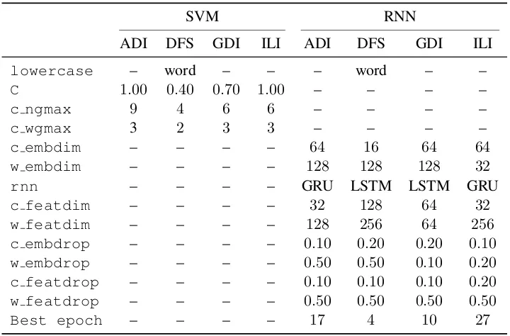
Table 3 presents the parameter settings that yielded best average macro-averaged F1 score based on

5-fold cross validation on the combined training and development sets. Although we report these values for the purpose of reproducibility, a rather large range of values result in similar performance scores. The distributions of F1 scores for both models are presented in Figure 1. The central tendency in box

plots presented in Figure 1 indicate that the F1score for many parameter settings for the SVM models

are close to the top score. Hence, a large range of ‘reasonable’ hyperparameter settings yield the scores similar to the top performing setting. The scores of the RNNs distributed more evenly (symmetrically), since they include a smaller number of randomly selected hyperparameter configurations.

We tune the hyperparameters which interact, for instance, both decreasingCand increasingmin df

may reduce overfitting. As a result, it is difficult to observe global trends of hyperparameter settings that yields better performance in a particular task. However, in general, frequency thresholds seems to hurt systems’ performances. The best performing hyperparameter settings used all features regardless of their frequencies (hence, frequency thresholds are not shown in Table 3).

3.3 Shared task results

During the evaluation campaign, we submitted predictions from the SVM and RNN models described above. In all the tasks, our SVM models were the best models among the ones for which we submitted predictions. Table 4 presents the macro-averaged precision, recall, and F1 scores of our SVM and RNN

models, as well as the official ranks obtained by the SVM model, and a rough indication of the rank of the RNN models assuming they were the only additional models to be included in the official rankings. For the ADI task, we only used the manually transcribed data, not making use of automatic transcriptions or audio features. The data presented in Table 4 also excludes the surprise dialect of the GDI task. We present results of the experiments on the surprise dialect conducted after the end of the shared task below. In general, our SVM system got the first rank on the DFS task, as well as ranking second or third on the other tasks. The scores of the RNN models are always behind the score of the SVMs, and the gap is particularly large for the ADI and ILI tasks.

The results on the test set presented in Table 4 are also drastically lower than the ones we obtained during development for some of the tasks, particularly for GDI and ADI, and to some extent for ILI. As presented in Table 5, the results on tests set is lower than the k-fold cross validation results on combined

SVM RNN

ADI DFS GDI ILI ADI DFS GDI ILI

lowercase – word – – – word – –

C 1.00 0.40 0.70 1.00 – – – –

c ngmax 9 4 6 6 – – – –

c wgmax 3 2 3 3 – – – –

c embdim – – – – 64 16 64 64

w embdim – – – – 128 128 128 32

rnn – – – – GRU LSTM LSTM GRU

c featdim – – – – 32 128 64 32

w featdim – – – – 128 256 64 256

c embdrop – – – – 0.10 0.20 0.20 0.10

w embdrop – – – – 0.50 0.50 0.10 0.20

c featdrop – – – – 0.10 0.10 0.10 0.20

w featdrop – – – – 0.50 0.50 0.50 0.50

Best epoch – – – – 17 4 10 27

Table 3: Best parameters for both SVM and RNN models tuned with 5-fold cross validation on the combined training and development data. The abbreviations for the parameters are explained in Table 2.

50 55 60 65 70 75 80 85 90 95 100

ADI DFS GDI ILI

Figure 1: Box plots showing the distribution of F1 scores obtained during the tuning process for the

SVM (blue, solid) and the RNN (dashed, red) models. The SVM scores include all hyperparameter values listed in Table 2, while the RNN scores only include approximately 40 random choices among indicated list of hyperparameters. Note that the RNN models have much lower number of data points and does not necessarily include the settings within the hyperparameter ranges that result in worst or best performance which may explain low variance in the RNN score distributions.

training and development sets with15.97 %,18.07 %, and7.27 %, for ADI, GDI, and ILI respectively, indicating a difference in distributions of training and the test sets. To check whether the designated development sets are closer to training or test sets, we also tuned the SVM models on the development set, whose results are also presented in Table 5. Indeed, for most data sets, the development sets seems to be closer to the test set. This may suggest that tuning the parameter values on the development sets rather than using k-fold cross validation may be better for obtaining better results in the shared task, despite its inferior performance to k-fold cross validation in an i.i.d. setting.

Task SVM RNN

Precision Recall F1-score Rank Precision Recall F1-score Rank

ADI 51.44 51.69 51.26 3 (5/ 6) 46.17 44.84 44.57 7

DFS 66.01 66.01 66.00 1 (1/11) 64.19 63.61 63.24 4

GDI 64.28 64.37 63.99 2 (4/ 8) 62.13 61.76 61.62 8

ILI 91.28 90.86 90.72 2 (2/ 8) 77.96 75.21 75.29 9

Table 4: Macro-averaged Precision, Recall, and F1-score of our SVM and RNN models. The scores of

the SVM models are the official results calculated by the organizers. The scores of the RNN models are calculated by us on the provided gold-standard test set. The ‘Rank’ column for the SVM lists the official rank based on statistically-significant differences, followed by the absolute rank and the number of participants for each task. The ‘Rank’ column of the RNN model is provided for a rough comparison and lists the absolute rank that would be obtained if the model were the only additional/unlisted model during the competition.

K-fold Dev-set Official

ADI 67.23 52.14 51.26

DFS 66.54 73.60 66.00

GDI 82.06 67.63 63.99

ILI 97.99 96.26 90.72

Table 5: The best F1-scores obtained during tuning with k-fold CV and using development set, as well as the official score. Clearly, there is a discrepancy between the full training set (k-fold results) and the test set for ADI and GDI. In the case of DFS, the development set seems to be closer to the training set. For ILI, the extent of the discrepancy seems to be smaller, but also development set is not necessarily closer to the test set than the training set.

5 %below the winning systems in ADI, GDI and ILI tasks respectively. The low performance of the system for the ADI is, however, expected since we did not make use of all the information. In general, the ILI task seems to be relatively easy, allowing over90 %F1 score on 5-way classification task. The

DFS task, on the other hand, seems more difficult. Although the classifiers certainly does much better than a random baseline, about66 %F1score is hardly impressive on a binary classification task.

3.4 Contribution of n-gram features

Our SVM models combine the word and character n-grams of various sizes. To investigate the usefulness of the individual n-gram features, we run a set of additional experiments, using only a limited set of features at a time. The results of these experiments are shown in Figure 2. The figure present the results of individual features (character or n-gram sizes) and combined features up to the indicated character or word n-gram order (e.g., the performance score corresponding to ‘combined’ trigrams include unigrams and bigrams of the indicated feature type). Across the datasets, we find that higher order features do not improve the results. In fact, we find that the F1scores drop rapidly when only higher-order n-grams are

used for both with character and word features.

For most data sets, performance of the systems peak for individual character ngrams of order4or5, after which usefulness of the higher order character n-grams start to degrade. It is also worth noting that even character unigrams are useful features across all data sets. The combined character n-gram features seem to yield slightly better scores than best-performing single n-gram order across the data sets, and with proper tuning, the additional, relatively useless features does not seem to hurt.

‘less-0 5 10 15 20 40 60 80 100 N-gram size F1 (macro) ADI single combined

0 5 10 15

20 40 60 80 100 N-gram size DFS

0 5 10 15

20 40 60 80 100 N-gram size GDI

0 5 10 15

20 40 60 80 100 N-gram size ILI

0 2 4 6 8

20 40 60 80 100 N-gram size F1 (macro) single combined

0 2 4 6 8

20 40 60 80 100 N-gram size

0 2 4 6 8

20 40 60 80 100 N-gram size

0 2 4 6 8

20 40 60 80 100 N-gram size

Figure 2: The macro averaged F1-scores for the SVM models using character (top) or word (bottom) n-gram of only the indicated n-gram size (blue lines with round markers) and up to the indicated n-gram size (red lines with triangle markers). The scores are the best macro-averaged F1scores obtained on the

combined training and development sets using 5-fold cross validation (averaged over 5 folds). Dashed horizontal lines indicate the expected scores of majority class baselines for each data set.

useful’ bigrams (or trigrams in case of ILI) seems to have a positive effect on the combined models. The GDI dataset presents an exception here. As well as slight performance drop when bigrams are combined with unigrams, higher-order word n-grams becomes less-informative, and degrades to majority baseline very quickly.

Figure 2 also indicates that character n-grams yield slightly better scores. This is also evident in the best F1 scores obtained by the character and word n-gram combinations presented in Table 6. We also

present the best setting that combines character and word n-grams for each dataset in Table 6. Although the character n-grams yield better results across all data sets, combining word n-grams is useful for DFS and GDI. Interestingly, despite the word n-grams seem least useful in the GDI task, the combination of character and word n-ngrams bring a noteworthy gain. In the ADI and the ILI tasks, we observe small performance loss when character and word n-grams are combined, compared to only using character n-grams.

3.5 GDI surprise dialect

ADI DFS GDI ILI

F1 c w F1 c w F1 c w F1 c w

Characters 67.28 7 0 65.98 6 0 81.42 8 0 98.05 7 0

Words 64.12 0 2 65.92 0 2 78.86 0 1 97.25 0 7

Characters and words 67.23 9 3 66.54 4 2 82.06 6 3 97.99 6 3

Table 6: Best macro-averaged F1scores obtained on the combined training/development set with 5-fold

cross validation with the SVM model. The column ‘c’ indicates the maximum character n-gram size and the column ‘w’ indicates maximum word n-gram size that yielded the corresponding score.

Decision rule No. of samples

predicted as XY Precision Recall F1-score

– (only four dialects) 0 44.02 51.48 47.39

Rejected by all 985 52.57 51.80 51.96

Accepted by several 413 46.80 49.36 47.74

Rejected or multi-accepted 1 398 52.91 49.62 50.51

Standard deviation 1 108 51.55 49.69 50.32

Difference 1 108 52.08 50.38 50.90

Table 7: Number of predictions for the surprise dialect ‘XY’ and macro-averaged precision, recall and F1-score of the SVM model for different decision criteria for predicting XY. We calculated the scores on the full gold-standard test set including the surprise dialect. The test set contains 790 XY samples out of 5542 samples total.

4 General discussion

As in earlier years, our participation in the VarDial 2018 shared task was based on two well-known classification methods, namely linear SVMs with bag-of-n-gram features, and recurrent ANN classifiers. Besides describing the systems, and presenting the official results, we also present a number of additional experiments and analysis of features used in our SVM models.

A common theme in our participation to VarDial has been the comparison between SVM and RNN classifiers. We and others have found SVMs to outperform RNNs in dialect / language identification tasks (C¸ ¨oltekin and Rama, 2016; C¸ ¨oltekin and Rama, 2017; Clematide and Makarov, 2017; Medvedeva et al., 2017), as well a few other text classification tasks (Rama and C¸ ¨oltekin, 2017; C¸ ¨oltekin and Rama, 2018; Malmasi and Dras, 2018). Similar to the results of the previous years, we found SVM models to work better than RNNs across all dialect identification tasks. Although in-line with earlier findings, the DFS task provided a possible advantage for RNNs, since the DFS data set is larger when compared to the other data sets, and large data is often considered one of the strengths of the deep learning methods. Our SVM model not only outperformed our RNN model, but also obtained the first place with an F1-score

difference of 1.50 % above the systems sharing the second place. Although RNNs are clearly behind SVMs also at the DFS task, the gap between RNNs and SVMs are smaller for DFS compared to ILI and ADI. One potential explanation, indeed, is the large data size. However, the GDI task, which has one of the smallest data sets, also exhibits a small performance difference similar to DFS task. A common trait of both the DFS and the GDI data sets is a more balanced text-length distribution (see Table 1), which may also be responsible for relatively better performance of the RNN models. However, more systematic experiments are required for identifying the conditions that affect the performances of the models.

pos-sible architectural improvements, performance of RNNs may be improved through data augmentation (Clematide and Makarov, 2017). Nevertheless, with their ‘baseline’ forms our present results support the earlier findings that in similar text classification tasks, SVMs with bag-of-n-gram features outperform the ANN classifiers based on gated RNN architectures.

With the SVM classifiers, it has been found earlier that character n-gram features perform well in lan-guage / dialect identification tasks (C¸ ¨oltekin and Rama, 2016; Bestgen, 2017). Our best submissions in this VarDial evaluation campaign were based on a combination of both character and word n-gram fea-tures which is supported through our analysis presented in Section 3.4. Moreover, the analysis also shows that depending on the task at hand, combining character n-gram features with word n-gram features may be helpful. The analysis in this section also shows that most of the gain in classification performance is based on rather low order features, character n-grams of order 4–5 and word uni- or bigrams seem to contain most valuable information while the higher order n-grams do not contribute much. This trend seems to persist with data sets with different size and properties, only with slight variation.

One of the interesting aspects of the present VarDial evaluation campaign has been the ‘surprise di-alect’ track of the GDI task. Although we did not submit results during the shared task due to time restrictions, we did a number of experiments with this task. Our results show that simple strategies based on assigning test instances where one-vs-rest multi-class classifiers are uncertain to the surprise dialect yields reasonable improvements. Particularly, assigning the test instances which were rejected by all of the one-vs-rest classifiers seems to perform the best in the present task.

5 Conclusions and outlook

In this paper we described our participation in the VarDial 2018 shared task. Our systems based on SVMs with bag-of-n-grams features ranked first in the DFS task, while obtaining second or third place in other language/dialect identification tasks. We reported scores of the alternative RNN classifier, presented analysis of usefulness of n-gram features in the SVM models, and also discussed possible strategies for predicting the surprise dialect in the GDI task.

Our results and analysis supports the earlier results that SVMs work better than RNNs in the tasks presented, and character (n-gram) features are seem to be most useful in SVM classifiers, while there may be small gains using both character and word n-gram features. Although we do not have a baseline to compare to at the time of this writing, our strategies for the surprise dialect also seem to bring reasonable improvements compared to not predicting the surprise dialect at all.

Although our models were successful during the shared task, they are ‘baseline’ models based on our participations in the earlier VarDial evaluation campaigns. There are a few straightforward points of improvements that can increase the performances of both the SVM and RNN models. For SVMs, one point of improvement is using a better feature weighting method than the sub-linear tf-idf used in this study. Another potentially useful direction for both SVMs and RNNs is the use of ensemble methods. This has been shown to work well with SVMs in earlier VarDial tasks. However, it is clearly not limited to the SVMs, it can be applied to RNNs too. Furthermore, since most ensemble methods work best when underlying classifiers are diverse, hybrid SVM-RNN ensembles are likely to perform even better. Last, but not the least, data augmentation methods are often shown to improve performance of deep learning methods such as RNNs. Although it is common to apply data augmentation for deep learning systems, investigating their effects on more ‘traditional’ models such as SVMs is another interesting possibility for improving results obtained with these models.

Acknowledgements

References

Mart´ın Abadi, Ashish Agarwal, Paul Barham, Eugene Brevdo, Zhifeng Chen, Craig Citro, Greg S. Corrado, Andy Davis, Jeffrey Dean, Matthieu Devin, Sanjay Ghemawat, Ian Goodfellow, Andrew Harp, Geoffrey Irving, Michael Isard, Yangqing Jia, Rafal Jozefowicz, Lukasz Kaiser, Manjunath Kudlur, Josh Levenberg, Dan Man´e, Rajat Monga, Sherry Moore, Derek Murray, Chris Olah, Mike Schuster, Jonathon Shlens, Benoit Steiner, Ilya Sutskever, Kunal Talwar, Paul Tucker, Vincent Vanhoucke, Vijay Vasudevan, Fernanda Vi´egas, Oriol Vinyals, Pete Warden, Martin Wattenberg, Martin Wicke, Yuan Yu, and Xiaoqiang Zheng. 2015. TensorFlow: Large-scale machine learning on heterogeneous systems. Software available from tensorflow.org.

Ahmed Ali, Najim Dehak, Patrick Cardinal, Sameer Khurana, Sree Harsha Yella, James Glass, Peter Bell, and Steve Renals. 2016. Automatic dialect detection in Arabic broadcast speech. In Proceedings of

INTER-SPEECH, pages 2934–2938.

Yves Bestgen. 2017. Improving the character ngram model for the DSL task with BM25 weighting and less frequently used feature sets. InProceedings of the Fourth Workshop on NLP for Similar Languages, Varieties and Dialects (VarDial), pages 115–123, Valencia, Spain, April.

C¸ a˘grı C¸ ¨oltekin and Taraka Rama. 2016. Discriminating similar languages with linear SVMs and neural networks. InProceedings of the Third Workshop on NLP for Similar Languages, Varieties and Dialects (VarDial3), pages 15–24, Osaka, Japan.

C¸ a˘grı C¸ ¨oltekin and Taraka Rama. 2017. T¨ubingen system in VarDial 2017 shared task: experiments with language identification and cross-lingual parsing. InProceedings of the Fourth Workshop on NLP for Similar Languages, Varieties and Dialects (VarDial), pages 146–155, Valencia, Spain.

Kyunghyun Cho, Bart van Merrienboer, Dzmitry Bahdanau, and Yoshua Bengio. 2014. On the properties of neural machine translation: Encoder–decoder approaches. In Proceedings of SSST-8, Eighth Workshop on Syntax, Semantics and Structure in Statistical Translation, pages 103–111.

Franc¸ois Chollet et al. 2015. Keras.https://github.com/keras-team/keras.

Simon Clematide and Peter Makarov. 2017. CLUZH at VarDial GDI 2017: Testing a variety of machine learning tools for the classification of swiss German dialects. InProceedings of the Fourth Workshop on NLP for Similar Languages, Varieties and Dialects (VarDial), pages 170–177, Valencia, Spain, April.

Rong-En Fan, Kai-Wei Chang, Cho-Jui Hsieh, Xiang-Rui Wang, and Chih-Jen Lin. 2008. LIBLINEAR: A library for large linear classification. Journal of Machine Learning Research, 9:1871–1874.

Sepp Hochreiter and J¨urgen Schmidhuber. 1997. Long short-term memory. Neural computation, 9(8):1735–1780.

Ritesh Kumar, Bornini Lahiri, Deepak Alok, Atul Kr. Ojha, Mayank Jain, Abdul Basit, and Yogesh Dawar. 2018. Automatic Identification of Closely-related Indian Languages: Resources and Experiments. InProceedings of

the Eleventh International Conference on Language Resources and Evaluation (LREC).

Shervin Malmasi and Mark Dras. 2018. Native language identification with classifier stacking and ensembles.

Computational Linguistics, (in press).

Shervin Malmasi and Marcos Zampieri. 2017a. Arabic dialect identification using iVectors and ASR transcripts. InProceedings of the Fourth Workshop on NLP for Similar Languages, Varieties and Dialects (VarDial), pages 178–183, Valencia, Spain, April.

Shervin Malmasi and Marcos Zampieri. 2017b. German dialect identification in interview transcriptions. In

Proceedings of the Fourth Workshop on NLP for Similar Languages, Varieties and Dialects (VarDial), pages

164–169, Valencia, Spain, April.

Shervin Malmasi, Marcos Zampieri, Nikola Ljubeˇsi´c, Preslav Nakov, Ahmed Ali, and J¨org Tiedemann. 2016. Discriminating between similar languages and Arabic dialect identification: A report on the third DSL shared task. InProceedings of the 3rd Workshop on Language Technology for Closely Related Languages, Varieties and Dialects (VarDial), Osaka, Japan.

Maria Medvedeva, Martin Kroon, and Barbara Plank. 2017. When sparse traditional models outperform dense neural networks: the curious case of discriminating between similar languages. InProceedings of the Fourth

Workshop on NLP for Similar Languages, Varieties and Dialects (VarDial), pages 156–163, Valencia, Spain,

F. Pedregosa, G. Varoquaux, A. Gramfort, V. Michel, B. Thirion, O. Grisel, M. Blondel, P. Prettenhofer, R. Weiss, V. Dubourg, J. Vanderplas, A. Passos, D. Cournapeau, M. Brucher, M. Perrot, and E. Duchesnay. 2011. Scikit-learn: Machine learning in Python. Journal of Machine Learning Research, 12:2825–2830.

Taraka Rama and C¸ a˘grı C¸ ¨oltekin. 2017. Fewer features perform well at native language identification task. In

Proceedings of the 12th Workshop on Innovative Use of NLP for Building Educational Applications, pages

255–260, Copenhagen, Denmark.

Tanja Samardˇzi´c, Yves Scherrer, and Elvira Glaser. 2016. ArchiMob–A corpus of spoken Swiss German. In

Proceedings of the Language Resources and Evaluation (LREC), pages 4061–4066, Portoroz, Slovenia).

Chris van der Lee and Antal van den Bosch. 2017. Exploring Lexical and Syntactic Features for Language Variety Identification. InProceedings of the Fourth Workshop on NLP for Similar Languages, Varieties and Dialects (VarDial), pages 190–199, Valencia, Spain.

Marcos Zampieri, Liling Tan, Nikola Ljubeˇsi´c, and J¨org Tiedemann. 2014. A report on the dsl shared task 2014.

In Proceedings of the First Workshop on Applying NLP Tools to Similar Languages, Varieties and Dialects

(VarDial), pages 58–67, Dublin, Ireland.

Marcos Zampieri, Shervin Malmasi, Nikola Ljubeˇsi´c, Preslav Nakov, Ahmed Ali, J¨org Tiedemann, Yves Scherrer, and No¨emi Aepli. 2017. Findings of the VarDial Evaluation Campaign 2017. InProceedings of the Fourth Workshop on NLP for Similar Languages, Varieties and Dialects (VarDial), Valencia, Spain.

Marcos Zampieri, Shervin Malmasi, Preslav Nakov, Ahmed Ali, Suwon Shuon, James Glass, Yves Scherrer, Tanja Samardˇzi´c, Nikola Ljubeˇsi´c, J¨org Tiedemann, Chris van der Lee, Stefan Grondelaers, Nelleke Oostdijk, Antal van den Bosch, Ritesh Kumar, Bornini Lahiri, and Mayank Jain. 2018. Language Identification and Morphosyntactic Tagging: The Second VarDial Evaluation Campaign. InProceedings of the Fifth Workshop on NLP for Similar Languages, Varieties and Dialects (VarDial), Santa Fe, USA.