Neural Lattice Language Models
Jacob Buckman
Language Technologies Institute Carnegie Mellon University [email protected]
Graham Neubig
Language Technologies Institute Carnegie Mellon University
Abstract
In this work, we propose a new language mod-eling paradigm that has the ability to perform both prediction and moderation of informa-tion flow at multiple granularities:neural lat-tice language models. These models con-struct a lattice of possible paths through a sen-tence and marginalize across this lattice to cal-culate sequence probabilities or optimize pa-rameters. This approach allows us to seam-lessly incorporate linguistic intuitions – in-cluding polysemy and the existence of multi-word lexical items – into our language model. Experiments on multiple language modeling tasks show that English neural lattice language models that utilize polysemous embeddings are able to improve perplexity by 9.95% rela-tive to a word-level baseline, and that a Chi-nese model that handles multi-character to-kens is able to improve perplexity by 20.94% relative to a character-level baseline.
1 Introduction
Neural network models have recently contributed to-wards a great amount of progress in natural language processing. These models typically share a common backbone: recurrent neural networks (RNN), which have proven themselves to be capable of tackling a variety of core natural language processing tasks (Hochreiter and Schmidhuber, 1997; Elman, 1990). One such task is language modeling, in which we estimate a probability distribution over sequences of tokens that corresponds to observed sentences (§2). Neural language models, particularly models con-ditioned on a particular input, have many applica-tions including in machine translation (Bahdanau et al., 2016), abstractive summarization (Chopra et al., 2016), and speech processing (Graves et al., 2013).
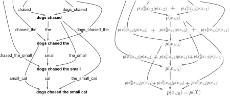
dogs chased the small cat dogs chased the small
cat dogs chased the
small dogs chased
the
the_small the_small_cat small_cat
dogs_chased chased
[image:1.612.308.533.184.280.2]chased_the dogs_chased_the chased_the_small
Figure 1: Lattice decomposition of a sentence and its cor-responding lattice language model probability calculation
Similarly, state-of-the-art language models are al-most universally based on RNNs, particularly long short-term memory (LSTM) networks (Jozefowicz et al., 2016; Inan et al., 2017; Merity et al., 2016).
While powerful, LSTM language models usually
do not explicitly model many commonly-accepted
linguistic phenomena. As a result, standard mod-els lack linguistically informed inductive biases, po-tentially limiting their accuracy, particularly in low-data scenarios (Adams et al., 2017; Koehn and Knowles, 2017). In this work, we present a novel modification to the standard LSTM language mod-eling framework that allows us to incorporate some varieties of these linguistic intuitions seamlessly:
neural lattice language models (§3.1). Neural lat-tice language models define a latlat-tice over possi-ble paths through a sentence, and maximize the marginal probability over all paths that lead to gen-erating the reference sentence, as shown in Fig. 1. Depending on how we define these paths, we can in-corporate different assumptions about how language should be modeled.
In the particular instantiations of neural lattice language models covered by this paper, we focus on two properties of language that could potentially be of use in language modeling: the existence of multi-word lexical units (Zgusta, 1967) (§4.1) and
poly-529
semy (Ravin and Leacock, 2000) (§4.2). Neural lat-tice language models allow the model to incorporate these aspects in an end-to-end fashion by simply ad-justing the structure of the underlying lattices.
We run experiments to explore whether these modifications improve the performance of the model (§5). Additionally, we provide qualitative visualiza-tions of the model to attempt to understand what types of multi-token phrases and polysemous em-beddings have been learned.
2 Background 2.1 Language Models
Consider a sequence X for which we want to
cal-culate its probability. Assume we have a vocabulary from which we can select a unique list of|X|tokens
x1, x2, . . . , x|X| such that X = [x1;x2;. . .;x|X|],
i.e. the concatenation of the tokens (with an appro-priate delimiter). These tokens can be either on the character level (Hwang and Sung, 2017; Ling et al., 2015) or word level (Inan et al., 2017; Merity et al., 2016). Using the chain rule, language models gen-erally factorizep(X)in the following way:
p(X) =p(x1, x2, . . . , x|X|)
=
|X|
Y
t=1
p(xt|x1, x2, . . . , xt−1). (1)
Note that this factorization is exact only in the case where the segmentation is unique. In character-level models, it is easy to see that this property is maintained, because each token is unique and non-overlapping. In word-level models, this also holds, because tokens are delimited by spaces, and no word contains a space.
2.2 Recurrent Neural Networks
Recurrent neural networks have emerged as the state-of-the-art approach to approximatingp(X). In
particular, the LSTM cell (Hochreiter and Schmid-huber, 1997) is a specific RNN architecture which has been shown to be effective on many tasks, in-cluding language modeling (Press and Wolf, 2017; Jozefowicz et al., 2016; Merity et al., 2016; Inan et
al., 2017).1 LSTM language models recursively
cal-1In this work, we utilize an LSTM with linked input and
forget gates, as proposed by Greff et al. (2016).
culate the hidden and cell states (ht andct
respec-tively) given the input embeddinget−1
correspond-ing to tokenxt−1:
ht, ct=LSTM(ht−1, ct−1, et−1, θ), (2)
then calculate the probability of the next token given the hidden state, generally by performing an affine
transform parameterized byW andb, followed by a
softmax:
p(xt|ht) :=softmax(W ∗ht+b). (3)
3 Neural Lattice Language Models 3.1 Language Models with Ambiguous
Segmentations
To reiterate, the standard formulation of language modeling in the previous section requires splitting sentenceXinto a unique set of tokensx1, . . . , x|X|.
Our proposed method generalizes the previous for-mulation to remove the requirement of uniqueness of segmentation, similar to that used in non-neural
n-gram language models such as Dupont and
Rosen-feld (1997) and Goldwater et al. (2007).
First, we define some terminology. We use the
term “token”, designated byxi, to describe any
in-divisible item in our vocabulary that has no other vocabulary item as its constituent part. We use the term “chunk”, designated by ki or xji, to describe a sequence of one or more tokens that represents a portion of the full stringX, containing the unit to-kens xi through xj: xji = [xi, xi+1;. . .;xj]. We also refer to the “token vocabulary”, which is the subset of the vocabulary containing only tokens, and to the “chunk vocabulary”, which similarly contains all chunks.
Note that we can factorize the probability of any
sequence of chunksK using the chain rule, in
pre-cisely the same way as sequences of tokens:
p(K) =p(k1, k2, . . . , k|K|)
=
|K|
Y
t=1
p(kt|k1, k2, . . . , kt−1). (4)
We can factorize the overall probability of a
to-ken listX in terms of its chunks by using the chain
segmentations S(X), such that for every sequence
s ∈ S(X), X = [xs1−1
s0 ;x
s2−1
s1 ;. . .;x
s|s|
s|s|−1]. The
factorization is:
p(X) =X S
p(X, S) =X S
p(X|S)p(S) = X S∈S(X)
p(S)
= X
S∈S(X) |S| Y
t=1
p(xst−1
st−1 |x s1−1 s0 , x
s2−1 s1 , . . . , x
st−1−1 st−2 ).
(5)
Note that, by definition, there exists a unique seg-mentation of X such thatx1, x2, . . . are all tokens,
in which case|S|=|X|. When only that one unique
segmentation is allowed perX,Scontains only that
one element, so summation drops out, and therefore for standard character-level and word-level models, Eq. (5) reduces to Eq. (4), as desired. However, for models that license multiple segmentations per
X, computing this marginalization directly is
gener-ally intractable. For example, consider segmenting a sentence using a vocabulary containing all words
and all 2-word expressions. The size of S would
grow exponentially with the number of words inX,
meaning we would have to marginalize over tril-lions of unique segmentations for even modestly-sized sentences.
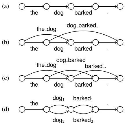
3.2 Lattice Language Models
To avoid this, it is possible to re-organize the com-putations in a lattice, which allows us to dramati-cally reduce the number of computations required (Dupont and Rosenfeld, 1997; Neubig et al., 2010).
All segmentations of X can be expressed as the
edges of paths through a lattice over token-level pre-fixes of X: x<1, x<2, . . . , X. The infimum is the
empty prefixx<1; the supremum isX; an edge from
prefix x<i to prefix x<j exists if and only if there exists a chunkxji in our chunk vocabulary such that
[x<i;xji] =x<j. Each path through the lattice from
x<1 toX is a segmentation ofXinto the list of
to-kens on the traversed edges, as seen in Fig. 1. The probability of a specific prefix p(x<j) is calculated by marginalizing over all segmentations leading up toxj−1
p(x<j) = X
S∈S(x<j)
|S|
Y
t=1
p(xst−1
st−1 |x<st−1), (6)
where by definitions|S| = j. The key insight here that allows us to calculate this efficiently is that this is a recursive formula and that instead of marginaliz-ing over all segmentations, we can marginalize over immediate predecessor edges in the lattice,Aj. Each item inAj is a locationi(= st−1), which indicates
that the edge between prefixx<iand prefixx<j, cor-responding to tokenxji, exists in the lattice. We can
thus calculatep(x<j)as
p(x<j) = X
i∈Aj
p(x<i)p(xji |x<i). (7)
SinceXis the supremum prefix node, we can use
this formula to calculatep(X) by setting j = |X|. In order to do this, we need to calculate the proba-bility of each of its|X|predecessors. Each of those
takes up to|X|calculations, meaning that the
com-putation forp(X)can be done in O(|X|2) time. If
we can guarantee that each node will have a
maxi-mum number of incoming edgesDso that|Aj| ≤D
for allj, then this bound can be reduced to O(D|X|)
time.2
The proposed technique is completely agnostic to the shape of the lattice, and Fig. 2 illustrates several potential varieties of lattices. Depending on how the lattice is constructed, this approach can be useful in a variety of different contexts, two of which we dis-cuss in§4.
3.3 Neural Lattice Language Models
There is still one missing piece in our attempt to ap-ply neural language models to lattices. Within our overall probability in Eq. (7), we must calculate the probability p(xji | x<i) of the next segment given the history. However, given that there are potentially an exponential number of paths through the lattice leading toxi, this is not as straightforward as in the
case where only one segmentation is possible. Pre-vious work on lattice-based language models (Neu-big et al., 2010; Dupont and Rosenfeld, 1997)
uti-lized count-basedn-gram models, which depend on
only a limited historical context at each step mak-ing it possible to compute the marginal probabilities in an exact and efficient manner through dynamic programming. On the other hand, recurrent neural
2Thus, the standard token-level language model whereD=
the dog barked .
the dog barked .
the dog dog barked .
the dog barked .
the dogdog barkedbarked .
the dog1 barked1 .
dog2 barked2
(a)
(b)
(c)
[image:4.612.79.295.52.265.2](d)
Figure 2: Example of (a) a single-path lattice, (b) a sparse lattice, (c) a dense lattice withD = 2, and (d) a
multilat-tice withD= 2, for sentence “the dog barked .”
models depend on the entire context, causing them to lack this ability. Our primary technical contribu-tion is therefore to describe several techniques for incorporating lattices into a neural framework with infinite context, by providing ways to approximate the hidden state of the recurrent neural net.
3.3.1 Direct Approximation
One approach to approximating the hidden state is the TreeLSTM framework described by Tai et al.
(2015).3 In the TreeLSTM formulation, new states
are derived from multiple predecessors by simply summing the individual hidden and cell state vec-tors of each of them. For each predecessor location
i ∈ Aj, we first calculate the local hidden state ˜h
and local cell statec˜by combining the embedding
eji with the hidden state of the LSTM at x<i using the standard LSTM update function as in Eq. (2):
˜
hi,˜ci =LSTM(hi, ci, eji, θ)fori∈Aj.
We then sum the local hidden and cell states:
hj =
X
i∈Aj
˜
hi cj =
X
i∈Aj
˜
ci.
3This framework has been used before for calculating neural
sentence representations involving lattices by Su et al. (2016) and Sperber et al. (2017), but not for the language models that are the target of this paper.
This formulation is powerful, but comes at the cost of sacrificing the probabilistic interpretation of which paths are likely. Therefore, even if almost all of the probability mass comes through the “true” segmentation, the hidden state may still be heavily influenced by all of the “bad” segmentations as well.
3.3.2 Monte-Carlo Approximation
Another approximation that has been proposed is to sample one predecessor state from all possible predecessors, as seen in Chan et al. (2017). We can calculate the total probability that we reach some
prefix x<j, and we know how much of this
prob-ability comes from each of its predecessors in the lattice, so we can construct a probability distribution over predecessors in the lattice:
M(x<i |θ) =
p(x<i |θ)p(xji |x<i;θ)
p(x<j |θ)
. (8)
Therefore, one way to update the LSTM is to sam-ple one predecessorx<ifrom the distributionMand simply sethj = ˜hiandcj = ˜ci. However, sampling is unstable and difficult to train: we found that the model tended to over-sample short tokens early on during training, and thus segmented every sentence into unigrams. This is similar to the outcome re-ported by Chan et al. (2017), who accounted for it
by incorporating anencouraging exploration.
3.3.3 Marginal Approximation
In another approach, which allows us to incorpo-rate information from all predecessors while main-taining a probabilistic interpretation, we can utilize
the probability distribution M to instead calculate
the expected value of the hidden state:
hj =Ex<i∼M[ ˜hi] =
X
i∈Aj
M(x<i|θ)˜hi
cj =Ex<i∼M[ ˜ci] =
X
i∈Aj
M(x<i|θ)˜ci.
3.3.4 Gumbel-Softmax Interpolation
the pre-softmax predecessor scores and then taking the argmax is equivalent to sampling from the prob-ability distribution. By replacing the argmax with a
softmax function scaled by a temperatureτ, we can
get this pseudo-sampled distribution through a fully differentiable computation:
N(x<i|θ) =
exp((log(M(x<i|θ)) +gi)/τ)
P
k∈Ajexp((log(M(x<k|θ)) +gk)/τ)
.
This new distribution can then be used to calculate the hidden state by taking a weighted average of the states of possible predecessors:
hj =
j−1
X
i∈Aj
N(x<i|θ)˜hi cj = j−1
X
i=j−L
N(x<i|θ)˜ci.
When τ is large, the values of N(x<i | θ) are flattened out; therefore, all the predecessor hidden states are summed with approximately equal weight, equivalent to the direct approximation (§3.3.1). On
the other hand, when τ is small, the output
distri-bution becomes extremely peaky, and one predeces-sor receives almost all of the weight. Each prede-cessorx<i has a chance of being selected equal to
M(x<i | θ), which makes it identical to ancestral sampling (§3.3.2). By slowly annealing the value of
τ, we can smoothly interpolate between these two
approaches, and end up with a probabilistic interpre-tation that avoids the instability of pure sampling-based approaches.
4 Instantiations of Neural Lattice LMs
In this section, we introduce two instantiations of neural lattice languages models aiming to capture features of language: the existence of coherent multi-token chunks, and the existence of polysemy.
4.1 Incorporating Multi-Token Phrases 4.1.1 Motivation
Natural language phrases often demonstrate sig-nificant non-compositionality: for example, in En-glish, the phrase “rock and roll” is a genre of mu-sic, but this meaning is not obtained by viewing the words in isolation. In word-level language model-ing, the network is given each of these words as in-put, one at a time; this means it must capture the id-iomaticity in its hidden states, which is quite round-about and potentially a waste of the limited param-eters in a neural network model. A straightforward
solution is to have an embedding for the entire multi-token phrase, and use this to input the entire phrase to the LSTM in a single timestep. However, it is also important that the model is able to decide whether the non-compositional representation is appropriate given the context: sometimes, “rock” is just a rock.
Additionally, by predicting multiple tokens in a single timestep, we are able to decrease the num-ber of timesteps across which the gradient must travel, making it easier for information to be prop-agated across the sentence. This is even more useful in non-space-delimited languages such as Chinese, in which segmentation is non-trivial, but character-level modeling leads to many sentences being hun-dreds of tokens long.
There is also psycho-linguistic evidence which supports the fact that humans incorporate multi-token phrases into their mental lexicon. Siyanova-Chanturia et al. (2011) show that native speakers of a language have significantly reduced response time when processing idiomatic phrases, whether they are used in an idiomatic sense or not, while Bannard and Matthews (2008) show that children learning a lan-guage are better at speaking common phrases than uncommon ones. This evidence lends credence to the idea that multi-token lexical units are a useful tool for language modeling in humans, and so may also be useful in computational models.
4.1.2 Modeling Strategy
The underlying lattices utilized in our multi-token phrase experiments are “dense” lattices: lattices
where every edge (below a certain length L) is
the missing edges, leading to wasted computation.
Since only edges of length L or less are present,
the maximum in-degree of any node in the lattice
D is no greater than L, giving us the time bound
O(L|X|).
4.1.3 Token Vocabularies
Storing an embedding for every possible
multi-token chunk would require |V|L unique
embed-dings, which is intractable. Therefore, we construct our multi-token embeddings by merging composi-tional and non-composicomposi-tional representations.
Non-compositional Representation We first es-tablish a priori set of “core” chunk-level tokens, each have a dense embedding. In order to guarantee full coverage of sentences, we first add every unit-level token to this vocabulary, e.g. every word in the cor-pus for a word-level model. Following this, we also
add the most frequent n-grams (where1 < n≤L).
This ensures that the vast majority of sentences will have several longer chunks appear within them, and so will be able to take advantage of tokens at larger granularities.
Compositional Representation However, the non-compositional embeddings above only account
for a subset of all n-grams, so we additionally
construct compositional embeddings for each chunk by running a BiLSTM encoder over the individual embeddings of each unit-level token within it (Dyer et al., 2016). In this way, we can create a unique embedding for every sequence of unit-level tokens.
We use this composition function on chunks regardless of whether they are assigned non-compositional embeddings or not, as even high-frequency chunks may display compositional prop-erties. Thus, for every chunk, we compute the chunk
embedding vectorxji by concatenating the
compo-sitional embedding with the non-compocompo-sitional em-bedding if it exists, or otherwise with an<UNK>
embedding.
Sentinel Mixture Model for Predictions At each
timestep, we want to use our LSTM hidden stateht
to assign some probability mass to every chunk with
a length less thanL. To do this, we follow Merity
et al. (2016) in creating a new “sentinel” token<s>
and adding it to our vocabulary. At each timestep,
we first use our neural network to calculate a score
for each chunkC in our vocabulary, including the
sentinel token. We do a softmax across these scores to assign a probabilitypmain(Ct+1 | ht;θ)to every chunk in our vocabulary, and also to<s>. For token
sequences not represented in our chunk vocabulary, this probabilitypmain(Ct+1 |ht;θ) = 0.
Next, the probability mass assigned to the sentinel value, pmain(<s> | ht;θ), is distributed across all
possible tokens sequences of length less thanL,
us-ing another LSTM with parametersθsub. Similar to
Jozefowicz et al. (2016), this sub-LSTM is initial-ized by passing in the hidden state of the main lattice LSTM at that timestep. This gives us a probability for each sequencepsub(c1, c2, . . . , cL|ht;θsub).
The final formula for calculating the probability
mass assigned to a specific chunkCis:
p(C |ht;θ) =pmain(C|ht;θ)+
pmain(<s>|ht;θ)psub(C|ht;θsub).
4.2 Incorporating Polysemous Tokens 4.2.1 Motivation
A second shortcoming of current language mod-eling approaches is that each word is associated with only one embedding. For highly polysemous words, a single embedding may be unable to represent all meanings effectively.
There has been past work in word embeddings which has shown that using multiple embeddings for each word is helpful in constructing a useful sentation. Athiwaratkun and Wilson (2017) repre-sented each word with a multimodal Gaussian dis-tribution and demonstrated that embeddings of this form were able to outperform more standard skip-gram embeddings on word similarity and entailment tasks. Similarly, Chen et al. (2015) incorporate standard skip-gram training into a Gaussian mixture framework and show that this improves performance on several word similarity benchmarks.
4.2.2 Modeling Strategy
For our polysemy experiments, the underlying lat-tices are latlat-tices: latlat-tices which are also multi-graphs, and can have any number of edges between any given pair of nodes (Fig. 2, d). Lattices set up in this manner allow us to incorporate multiple em-beddings for each word. Within a single sentence, any pair of nodes corresponds to the start and end of a particular subsequence of the full sentence, and is thus associated with a specific token. Each edge between them is a unique embedding for that to-ken. While many strategies for choosing the num-ber of embeddings exist in the literature (Neelakan-tan et al., 2014), in this work, we choose a number
of embeddingsE and assign that many embeddings
to each word. This ensures that the maximum
in-degree of any node in the lattice D, is no greater
thanE, giving us the time bound O(E|X|).
In this work, we do not explore models that in-clude both chunk vocabularies and multiple embed-dings. However, combining these two techniques, as well as exploring other, more complex lattice struc-tures, is an interesting avenue for future work.
5 Experiments 5.1 Data
We perform experiments on two languages: English and Chinese, which provide an interesting contrast in linguistic features.4
In English, the most common benchmark for language modeling recently is the Penn Tree-bank, specifically the version preprocessed by Tom´aˇs Mikolov (2010). However, this corpus is lim-ited by being relatively small, only containing ap-proximately 45,000 sentences, which we found to be insufficient to effectively train lattice language
mod-els.5 Thus, we instead used the Billion Word Corpus
(Chelba et al., 2014). Past experiments on the BWC typically modeled every word without restricting the vocabulary, which results in a number of challenges regarding the modeling of open vocabularies that are orthogonal to this work. Thus, we create a
pre-4Code to reproduce datasets and experiments is
available at: http://github.com/jbuckman/ neural-lattice-language-models
5Experiments using multi-word units resulted in overfitting,
regardless of normalization and hyperparameter settings.
processed version of the data in the same manner as Mikolov, lowercasing the words, replacing num-bers with<N>tokens, and<UNK>ing all words
beyond the ten thousand most common. Addition-ally, we restricted the data set to only include sen-tences of length 50 or less, ensuring that large mini-batches could fit in GPU memory. Our subsampled English corpus contained 29,869,166 sentences, of which 29,276,669 were used for training, 5,000 for validation, and 587,497 for testing. To validate that our methods scale up to larger language modeling scenarios, we also report a smaller set of large-scale experiments on the full billion word benchmark in Appendix A.
In Chinese, we ran experiments on a subset of the Chinese GigaWord corpus. Chinese is also par-ticularly interesting because unlike English, it does not use spaces to delimit words, so segmentation is non-trivial. Therefore, we used a character-level lan-guage model for the baseline, and our lattice was composed of multi-character chunks. We used
sen-tences from Guangming Daily, again <UNK>ing
all but the 10,000 most common tokens and restrict-ing the selected sentences to only include sentences of length 150 or less. Our subsampled Chinese cor-pus included 934,101 sentences for training, 5,000 for validation, and 30,547 for testing.
5.2 Main Experiments
We compare a baseline LSTM model, dense lattices of size 1, 2, and 3, and a multilattice with 2 and 3 embeddings per word.
The implementation of our networks was done in DyNet (Neubig et al., 2017). All LSTMs had 2 lay-ers, each with a hidden dimension of 200. Vari-ational dropout (Gal and Ghahramani, 2016) of .2 was used on the Chinese experiments, but hurt per-formance on the English data, so it was not used. The 10,000 word embeddings each had dimension 256. For lattice models, chunk vocabularies were se-lected by taking the 10,000 words in the vocabulary
and adding the most common 10,000n-grams with
1< n≤L. The weights on the final layer of the
net-work were tied with the input embeddings, as done by Press and Wolf (2017) and Inan et al. (2017). In all lattice models, hidden states were computed
using a weighted expectation (§3.3.3) unless
em-Table 1: Results on English language modeling task
Model Valid. Perp. Test Perp.
Baseline 47.64 48.62
Multi-Token (L= 1) 45.69 47.21
Multi-Token (L= 2) 44.15 46.12
Multi-Token (L= 3) 45.19 46.84
Multi-Emb (E = 2) 44.80 46.32
[image:8.612.73.299.72.180.2]Multi-Emb (E = 3) 42.76 43.78
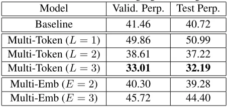
Table 2: Results on Chinese language modeling task
Model Valid. Perp. Test Perp.
Baseline 41.46 40.72
Multi-Token (L= 1) 49.86 50.99
Multi-Token (L= 2) 38.61 37.22
Multi-Token (L= 3) 33.01 32.19
Multi-Emb (E = 2) 40.30 39.28
Multi-Emb (E = 3) 45.72 44.40
bedding sizes were decreased so as to maintain the same total number of parameters. All models were trained using the Adam optimizer with a learning rate of .01 on a NVIDIA K80 GPU. The results can be seen in Table 1 and Table 2.
In the multi-token phrase experiments, many ad-ditional parameters are accrued by the BiLSTM encoder and sub-LSTM predictive model, making them not strictly comparable to the baseline. To
ac-count for this, we include results forL = 1, which,
like the baseline LSTM approach, fails to leverage multi-token phrases, but includes the same number
of parameters asL= 2andL= 3.
In both the English and Chinese experiments, we see the same trend: increasing the maximum
lat-tice size decreases the perplexity, and for L = 2
and above, the neural lattice language model outper-forms the baseline. Similarly, increasing the number of embeddings per word decreases the perplexity,
and forE = 2and above, the multiple-embedding
model outperforms the baseline.
5.3 Hidden State Calculation Experiments
We compare the various hidden-state calculation ap-proaches discussed in Section 3.3 on the English
data using a lattice of size L = 2 and dropout of
[image:8.612.315.539.74.153.2].2. These results can be seen in Table 3.
Table 3: Hidden state calculation comparison results Model Valid. Perp. Test Perp.
Baseline 64.18 60.67
Direct (§3.3.1) 59.74 55.98 Monte Carlo (§3.3.2) 62.97 59.08 Marginalization (§3.3.3) 58.62 55.06 GS Interpolation (§3.3.4) 59.19 55.73
For all hidden state calculation techniques, the neural lattice language models outperform the LSTM baseline. The ancestral sampling technique used by Chan et al. (2017) is worse than the others, which we found to be due to it getting stuck in a lo-cal minimum which represents almost everything as unigrams. There is only a small difference between the perplexities of the other techniques.
5.4 Discussion and Analysis
Neural lattice language models convincingly out-perform an LSTM baseline on the task of lan-guage modeling. One interesting note is that in En-glish, which is already tokenized into words and highly polysemous, utilizing multiple embeddings per word is more effective than including multi-word tokens. In contrast, in the experiments on the Chinese data, increasing the lattice size of the multi-character tokens is more important than increasing the number of embeddings per character. This cor-responds to our intuition; since Chinese is not tok-enized to begin with, utilizing models that incorpo-rate segmentation and compositionality of elemen-tary units is very important for effective language modeling.
To calculate the probability of a sentence, the neural lattice language model implicitly marginal-izes across latent segmentations. By inspecting the probabilities assigned to various edges of the lattice, we can visualize these segmentations, as is done in Fig. 3. The model successfully identifies bi-grams which correspond to non-compositional com-pounds, like “prime minister”, and bigrams which correspond to compositional compounds, such as “a quarter”. Interestingly, this does not occur for all high-frequency bigrams; it ignores those that are not inherently meaningful, such as “<UNK>in”,
yield-ing qualitatively good phrases.
[image:8.612.72.298.210.318.2]pos-Figure 3: Segmentation of three sentences randomly sampled from the test corpus, usingL= 2. Green numbers show
[image:9.612.101.488.55.150.2]probability assigned to token sizes. For example, the first three words in the first sentence have a 59% and 41% chance of being “please let me” or “please let me” respectively. Boxes around words show greedy segmentation.
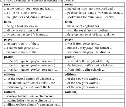
Table 4: Comparison of randomly-selected contexts of several words selected from the vocabulary of the Billion Word Corpus, in which the model preferred one embedding over the other.
rock1 rock2
...at the<unk>pop ,rockand jazz... ...including hsbc , northernrockand...
...a little bit<unk>rock,... ...pakistan has a<unk>rockmusic scene...
...on lightrockand<unk>stations... ...spokesman for roundrock,<unk>...
bank1 bank2
...being abankholiday in... ...thebankof england has...
...all the usbankruns and... ...with the royalbankof scotland...
...by getting thebank’s interests... ...developmentbankof japan and the...
page1 page2
...onpage<unk>of the... ...was it frontpagenews...
...a source toldpagesix .... ...himself , tonypage, the former ...
...onpage<unk>of the... ...sections of thepagethat discuss...
profile1 profile2
...(<unk>: quote ,profile, research )... ...so<unk>theprofileof the city...
...(<unk>: quote ,profile, research )... ...the highestprofile<unk>held by...
...(<unk>: quote ,profile, research )... ...from high i , elite schools ,...
edition1 edition2
... of the secondeditionof windows... ...of the new yorkedition. ...
... this month ’seditionof<unk>, the ... ...of the new yorkedition. ...
...forthcoming d.c.editionof the hit... ...of the new yorkedition. ...
rodham1 rodham2
...senators hillaryrodhamclinton and... ...making hillaryrodhamclinton his...
...hillaryrodhamclinton ’s campaign has...
sible to see which of the two embeddings of a word was assigned the higher probability for any specific test-set sentence. In order to visualize what types of meanings are assigned to each embedding, we select sentences in which one embedding is preferred, and look at the context in which the word is used.
[image:9.612.97.512.239.592.2]con-text in which they appear. In some cases, likeprofile
andedition, one of the two embeddings simply cap-tures an idiosyncrasy of the training data.
Additionally, for some words, such asrodhamin
Table 4, the system always prefers one embedding. This is promising, because it means that in future work it may be possible to further improve accu-racy and training efficiency by assigning more em-beddings to polysemous words, instead of assigning the same number of embeddings to all words.
6 Related Work
Past work that utilized lattices in neural models for natural language processing centers around us-ing these lattices in the encoder portion of machine translation. Su et al. (2016) utilized a variation of the Gated Recurrent Unit (GRU) that operated over lattices, and preprocessed lattices over Chi-nese characters that allowed it to effectively encode multiple segmentations. Additionally, Sperber et al. (2017) proposed a variation of the TreeLSTM with the goal of creating an encoder over speech lattices in speech-to-text. Our work tackles language mod-eling rather than encoding, and thus addresses the issue of marginalization over the lattice.
Another recent work which marginalized over multiple paths through a sentence is Ling et al. (2016). The authors tackle the problem of code gen-eration, where some components of the code can be copied from the input, via a neural network. Our work expands on this by handling multi-word tokens as input to the neural network, rather than passing in one token at a time.
Neural lattice language models improve accuracy by helping the gradient flow over smaller paths, pre-venting vanishing gradients. Many hierarchical neu-ral language models have been proposed with a sim-ilar objective (Koutnik et al., 2014; Zhou et al., 2017). Our work is distinguished from these by the use of latent token-level segmentations that cap-ture meaning directly, rather than simply being high-level mechanisms to encourage gradient flow.
Chan et al. (2017) propose a model for predict-ing characters at multiple granularities in the de-coder segment of a machine translation system. Our work expands on theirs by considering the entire lat-tice at once, rather than considering a only a
sin-gle path through the lattice via ancestral sampling. This allows us to train end-to-end without the model collapsing to a local minimum, with no exploration bonus needed. Additionally, we propose a more broad class of models, including those incorporat-ing polysemous words, and apply our model to the task of word-level language modeling, rather than character-level transcription.
Concurrently to this work, van Merri¨enboer et al. (2017) have proposed a neural language model that can similarly handle multiple scales. Our work is differentiated in that it is more general: utilizing an open multi-token vocabulary, proposing multiple techniques for hidden state calculation, and handling polysemy using multi-embedding lattices.
7 Future Work
In the future, we would like to experiment with uti-lizing neural lattice language models in extrinsic evaluation, such as machine translation and speech recognition. Additionally, in the current model, the non-compositional embeddings must be selected a priori, and may be suboptimal. We are exploring techniques to store fixed embeddings dynamically, so that the non-compositional phrases can be se-lected as part of the end-to-end training.
8 Conclusion
In this work, we have introduced the idea of a neural lattice language model, which allows us to marginal-ize over all segmentations of a sentence in an end-to-end fashion. In our experiments on the Billion Word Corpus and Chinese GigaWord corpus, we demonstrated that the neural lattice language model beats an LSTM-based baseline at the task of lan-guage modeling, both when it is used to incorpo-rate multiple-word phrases and multiple-embedding words. Qualitatively, we observed that the latent segmentations generated by the model correspond well to human intuition about multi-word phrases, and that the varying usage of words with multiple embeddings seems to also be sensible.
Acknowledgements
References
Oliver Adams, Adam Makarucha, Graham Neubig, Steven Bird, and Trevor Cohn. 2017. Cross-lingual word embeddings for low-resource language model-ing. InProceedings of the 15th Conference of the Eu-ropean Chapter of the Association for Computational Linguistics: Volume 1, Long Papers, volume 1, pages 937–947.
Ben Athiwaratkun and Andrew Wilson. 2017. Multi-modal word distributions. InProceedings of the 55th Annual Meeting of the Association for Computational Linguistics (Volume 1: Long Papers), volume 1, pages 1645–1656.
Dzmitry Bahdanau, Jan Chorowski, Dmitriy Serdyuk, Philemon Brakel, and Yoshua Bengio. 2016. End-to-end attention-based large-vocabulary speech recog-nition. In IEEE International Conference on Acous-tics, Speech and Signal Processing, pages 4945–4949. IEEE.
Colin Bannard and Danielle Matthews. 2008. Stored word sequences in language learning: The effect of familiarity on children’s repetition of four-word com-binations.Psychological Science, 19(3):241–248. William Chan, Yu Zhang, Quoc Le, and Navdeep Jaitly.
2017. Latent sequence decompositions. 5th Interna-tional Conference on Learning Representations. Ciprian Chelba, Tomas Mikolov, Mike Schuster, Qi Ge,
Thorsten Brants, Phillipp Koehn, and Tony Robinson. 2014. One billion word benchmark for measuring progress in statistical language modeling. Interspeech. Xinchi Chen, Xipeng Qiu, Jingxiang Jiang, and Xuanjing Huang. 2015. Gaussian mixture embeddings for mul-tiple word prototypes. CoRR, abs/1511.06246. Sumit Chopra, Michael Auli, Alexander M Rush, and
SEAS Harvard. 2016. Abstractive sentence sum-marization with attentive recurrent neural networks.
North American Chapter of the Association for Com-putational Linguistics: Human Language Technolo-gies, pages 93–98.
Pierre Dupont and Ronald Rosenfeld. 1997. Lattice based language models. Technical report, DTIC Doc-ument.
Chris Dyer, Adhiguna Kuncoro, Miguel Ballesteros, and Noah A Smith. 2016. Recurrent neural network gram-mars. North American Chapter of the Association for Computational Linguistics: Human Language Tech-nologies, pages 199–209.
Jeffrey L. Elman. 1990. Finding structure in time. Cog-nitive science, 14(2):179–211.
Yarin Gal and Zoubin Ghahramani. 2016. A theoreti-cally grounded application of dropout in recurrent neu-ral networks. InAdvances in Neural Information Pro-cessing Systems, pages 1019–1027.
Sharon Goldwater, Thomas L. Griffiths, Mark Johnson, et al. 2007. Distributional cues to word boundaries: Context is important. In H. Caunt-Nulton, S. Kilati-late, and I. Woo, editors,BUCLD 31: Proceedings of the 31st Annual Boston University Conference on Lan-guage Development, pages 239–250. Somerville, Mas-sachusetts: Cascadilla Press.
Alex Graves, Abdel-rahman Mohamed, and Geoffrey Hinton. 2013. Speech recognition with deep recurrent neural networks. InIEEE International Conference on Acoustics, Speech and Signal Processing, pages 6645– 6649. IEEE.
Klaus Greff, Rupesh K. Srivastava, Jan Koutn´ık, Bas R. Steunebrink, and J¨urgen Schmidhuber. 2016. LSTM: A search space odyssey. IEEE Transactions on Neural Networks and Learning Systems.
Sepp Hochreiter and J¨urgen Schmidhuber. 1997. Long short-term memory. Neural Computation, 9(8):1735– 1780.
Kyuyeon Hwang and Wonyong Sung. 2017. Character-level language modeling with hierarchical recurrent neural networks. InIEEE International Conference on Acoustics, Speech and Signal Processing, pages 5720– 5724. IEEE.
Hakan Inan, Khashayar Khosravi, and Richard Socher. 2017. Tying word vectors and word classifiers: A loss framework for language modeling. 5th International Conference on Learning Representations.
Eric Jang, Shixiang Gu, and Ben Poole. 2017. Categori-cal reparameterization with Gumbel-Softmax. 5th In-ternational Conference on Learning Representations. Rafal Jozefowicz, Oriol Vinyals, Mike Schuster, Noam
Shazeer, and Yonghui Wu. 2016. Exploring the limits of language modeling. arXiv:1602.02410.
Philipp Koehn and Rebecca Knowles. 2017. Six chal-lenges for neural machine translation. InProceedings of the First Workshop on Neural Machine Translation, pages 28–39.
Jan Koutnik, Klaus Greff, Faustino Gomez, and Juergen Schmidhuber. 2014. A clockwork RNN. Proceedings of Machine Learning Research.
Wang Ling, Isabel Trancoso, Chris Dyer, and Alan W. Black. 2015. Character-based neural machine transla-tion. CoRR, abs/1511.04586.
Wang Ling, Edward Grefenstette, Karl Moritz Hermann, Tom´aˇs Koˇcisk`y, Andrew Senior, Fumin Wang, and Phil Blunsom. 2016. Latent predictor networks for code generation. Association for Computational Lin-guistics.
Stephen Merity, Caiming Xiong, James Bradbury, and Richard Socher. 2016. Pointer sentinel mixture mod-els. 4th International Conference on Learning Repre-sentations.
Arvind Neelakantan, Jeevan Shankar, Re Passos, and An-drew Mccallum. 2014. Efficient nonparametric es-timation of multiple embeddings per word in vector space. InProceedings of EMNLP. Citeseer.
Graham Neubig, Masato Mimura, Shinsuke Mori, and Tatsuya Kawahara. 2010. Learning a language model from continuous speech. In INTERSPEECH, pages 1053–1056.
Graham Neubig, Chris Dyer, Yoav Goldberg, Austin Matthews, Waleed Ammar, Antonios Anastasopoulos, Miguel Ballesteros, David Chiang, Daniel Clothiaux, Trevor Cohn, et al. 2017. DyNet: The dynamic neural network toolkit. arXiv preprint arXiv:1701.03980. Ofir Press and Lior Wolf. 2017. Using the output
embed-ding to improve language models. 5th International Conference on Learning Representations.
Yael Ravin and Claudia Leacock. 2000. Polysemy: The-oretical and Computational Approaches. OUP Ox-ford.
Rico Sennrich, Barry Haddow, and Alexandra Birch. 2015. Neural machine translation of rare words with subword units. Association for Computational Lin-guistics.
Anna Siyanova-Chanturia, Kathy Conklin, and Norbert Schmitt. 2011. Adding more fuel to the fire: An eye-tracking study of idiom processing by native and non-native speakers. Second Language Research, 27(2):251–272.
Matthias Sperber, Graham Neubig, Jan Niehues, and Alex Waibel. 2017. Neural lattice-to-sequence mod-els for uncertain inputs. InProceedings of the 2017 Conference on Empirical Methods in Natural Lan-guage Processing, pages 1380–1389.
Jinsong Su, Zhixing Tan, Deyi Xiong, and Yang Liu. 2016. Lattice-based recurrent neural net-work encoders for neural machine translation. CoRR, abs/1609.07730, ver. 2.
Kai Sheng Tai, Richard Socher, and Christopher D. Man-ning. 2015. Improved semantic representations from tree-structured long short-term memory networks. As-sociation for Computational Linguistics.
Luk´aˇs Burget Jan Honza Cernock Sanjeev Khudanpur Tom´aˇs Mikolov, Martin Karafi´at. 2010. Recur-rent neural network based language model. Pro-ceedings of the 11th Annual Conference of the Inter-national Speech Communication Association, pages 1045–1048.
Bart van Merri¨enboer, Amartya Sanyal, Hugo Larochelle, and Yoshua Bengio. 2017. Multiscale sequence
modeling with a learned dictionary. arXiv preprint arXiv:1707.00762.
Ladislav Zgusta. 1967. Multiword lexical units. Word, 23(1-3):578–587.
Hao Zhou, Zhaopeng Tu, Shujian Huang, Xiaohua Liu, Hang Li, and Jiajun Chen. 2017. Chunk-based bi-scale decoder for neural machine translation. Associa-tion for ComputaAssocia-tional Linguistics.
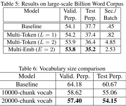
A Large-Scale Experiments
To verify that our findings scale to state-of-the-art language models, we also compared a baseline model, dense lattices of size 1 and 2, and a multi-lattice with 2 embeddings per word on the full byte-pair encoded Billion Word Corpus.
In this set of experiments, we take the full Bil-lion Word Corpus, and apply byte-pair encoding as described by Sennrich et al. (2015) to construct a vocabulary of 10,000 sub-word tokens. Our model consists of three LSTM layers, each with 1500 hid-den units. We train the model for a single epoch over the corpus, using the Adam optimizer with learning rate .0001 on a P100 GPU. We use a batch size of 40, and variational dropout of 0.1. The 10,000 sub-word embeddings each had dimension 600. For lattice models, chunk vocabularies were selected by taking the 10,000 sub-words in the vocabulary and adding
the most common 10,000n-grams with1< n≤L.
The weights on the final layer of the network were tied with the input embeddings, as done by Press and Wolf (2017) and Inan et al. (2017). In all lattice models, hidden states were computed using weighted expectation (§3.3.3). In multi-embedding models, embedding sizes were decreased so as to maintain the same total number of parameters.
Table 5: Results on large-scale Billion Word Corpus
Model Valid. Test Sec./
Perp. Perp. Batch
Baseline 54.1 37.7 .45
Multi-Token (L= 1) 54.2 37.4 .82
Multi-Token (L= 2) 53.9 36.4 4.85
Multi-Emb (E= 2) 53.8 35.2 2.53
Table 6: Vocabulary size comparison
Model Valid. Perp. Test Perp.
Baseline 64.18 60.67
10000-chunk vocab 58.62 55.06
20000-chunk vocab 57.40 54.15
B Chunk Vocabulary Size