Parameter Free Hierarchical Graph-Based Clustering for Analyzing
Continuous Word Embeddings
Thomas A. Trost Dietrich Klakow Saarland University
Saarbr¨ucken, Germany
{thomas.trost,dietrich.klakow}@lsv.uni-saarland.de
Abstract
Word embeddings are high-dimensional vector representations of words and are thus difficult to interpret. In order to deal with this, we introduce an unsupervised parameter free method for creating a hi-erarchical graphical clustering of the full ensemble of word vectors and show that this structure is a geometrically meaning-ful representation of the original relations between the words. This newly obtained representation can be used for better un-derstanding and thus improving the em-bedding algorithm and exhibits semantic meaning, so it can also be utilized in a va-riety of language processing tasks like cat-egorization or measuring similarity.
1 Introduction
There are different ways to assess word embed-dings (Yaghoobzadeh and Sch¨utze,2016). While some authors focus on general properties, as for example Levy et al. (2015) or Hashimoto et al. (2016), most evaluations are with respect to spe-cific tasks. Examples of the latter include the works by Baroni et al. (2014), Schnabel et al. (2015), orRothe and Sch¨utze(2016), to name but a few. The objective of this paper is to intro-duce a method for getting a grasp of the global
structure of embeddings, which is different from general schemes for dimensionality reduction like t-SNE (Maaten and Hinton, 2008), the methods summarized byVan Der Maaten et al.(2009), or visualization interfaces such as Roleo (Sayeed et al.,2016) andGoWvis(Tixier et al.,2016). The method presented here is a specific way of cluster-ing (a field nicely reviewed byJain et al.(1999)) that works particularly well for the current objec-tive.
We present a global analysis of the statistical properties of the embedding space. This is based on the output of the well-knownword2vec pro-gram (Mikolov et al., 2013), using the example of the dataset published alongside the source code on the web1, which was generated with the
skip-gram model with negative sampling. This dataset was trained on parts of the English Google news corpus and consists of 3,000,000 words with 300-dimensional embedding vectors. First, densities in the embedding space will be explored. Based on that a parameter free hierarchical graph-based clustering approach is developed that is the basis of a tool that allows to explore the neighborhood of a term of interest.
The paper is structured as follows: After a quick discussion of statistical properties of the dataset, the concept of the graphical neighborhood hierar-chy is explained. Specific properties of the result-ing graphs are brought into the context of pecu-liarities of the dataset for showing that this repre-sentation is particularly well-suited. Finally, the semantic properties of the graphs are briefly eval-uated.
2 Properties of Embedding Spaces
First, a look at global statistics of the dataset lays a basis for justifying later choices and interpreting the hierarchy. Herein, special care must be taken with respect to effects of the high dimensionality.
The distribution of the values of single vector components all look very similar and peak clearly at the origin, but they exhibit relatively heavy tails. The distribution of theL2-norm2of the embedding vectors can be seen in fig.1, both for all and rare words, where the latter are those that are not found
1https://code.google.com/archive/p/ word2vec/
2For a discussion of the choice of distance function, see section3.2below.
in the1 billion wordcorpus (Chelba et al.,2013). Even though the curves show a drop at the origin
0 0.2 0.4 0.6
0 1 2 3 4 5 6 7
100
10−300 10−200 10−100 10100 10200 10300
[image:2.595.77.279.105.212.2]L2-norm prob. dens. (all) prob. dens. (rare) average density
Figure 1: Probability densitiesfor finding a word vector with the given norm, for all and rare words (left axis, density for rare words rescaled for re-flecting proportion) and plot of the resulting aver-age densityat the respective distance to the origin (right axis).
and a clear peak at slightly above one, they are mostly a consequence of the high dimensionality of the embedding space. This becomes apparent in the plot of the actual average density (words per volume) at a given distance from the origin (also fig. 1), which decreases very rapidly and mono-tonically. It can be concluded that embedding vec-tors are highly concentrated around the origin, but that common words tend to lie at an intermediate distance to the origin and do not fully follow the general distribution.
Next, a principle component analysis can be done in order to evaluate how isotropic the dataset actually is. It reveals that the largest and smallest eigenvalues are only about an order of magnitude apart and that the top 20 percent of eigenvalues account for roughly 50 percent of the total vari-ance in the dataset. While this is clearly not fully isotropic, there appear to be no directions that are completely superfluous. For the global picture, ap-proximate isotropy is thus a fairly reasonable as-sumption.
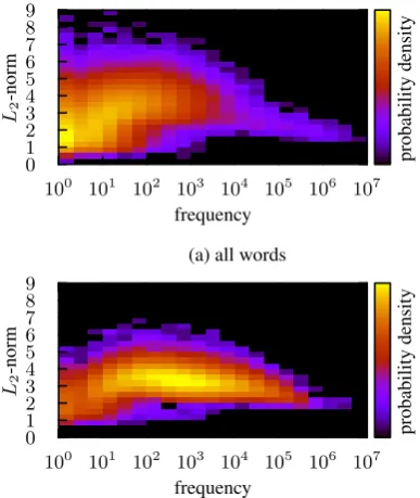
To complete the general statistical exploration of the embedding space we want to look at spe-cific word classes (common nouns, verbs and ad-jectives) versus other words that belong to none of these classes. We also want to explore the impact of the word frequency on the position in the em-bedding space. Figure2gives the results. The first – however non-surprising – observation is that the center of the embedding space is made up of low frequency words that are not nouns, verbs or ad-jectives. These three POS classes densely
popu-late the surface of a 300 dimensional sphere in a distance of three to four from the center of the em-bedding space. Exploring this rim in more detail is most interesting for applications. For this we will develop a parameter free method to study the vicinity of a word of interest to the user of the tool.
100 101 102 103 104 105 106 107 frequency
0 1 2 3 4 5 6 7 8 9
L2
-norm
probability
density
(a) all words
100 101 102 103 104 105 106 107 frequency
0 1 2 3 4 5 6 7 8 9
L2
-norm
probability
density
(b) common nouns, verbs, and adjectives Figure 2: Probability density for finding an em-bedding vector of a word of given frequency and a givenL2-norm and thus distance from the origin. Note that the density is given in log-scale.
3 Nearest Neighbor Graph
Consider a set of embedding vectors W that is equipped with a distance functiond:W × W →
R+0. The nearest neighbor graph (NNG) on W
is a directed weighted graph where each vertexv has outdegree one and is connected to its nearest neighborw= arg minw0d(v, w0), with the weight
corresponding to the distance. In case of ambi-guity, the nearest neighbor has to be selected via additional criteria or randomly. Note that the near-est neighbor relation need not be reciprocal. The k-NNG which incorporates the notion ofk near-est neighbors can be defined in a similar way, but it lacks most of the nice properties of the simple NNG, some of which will be discussed next.
[image:2.595.311.505.159.389.2]efficiency depends on the dimensionality of W. Thus, in particular for high-dimensional spaces, approximate nearest neighbor search may be much more efficient (Muja and Lowe,2009).
3.1 Clusters
Here, the weakly connected components of an NNG are denoted asclusters. That is to say, there is a path between every two vertices within a clus-ter, if the direction of the edges is ignored. It can readily be seen that each cluster must have exactly one cluster root, which is a pair of vertices that see each other as their nearest neighbor. Apart from that, there cannot be any cycles in a cluster, so it can be considered as two trees each of which is rooted in one vertex of the cluster root. This tree-like and very clear structure of the clusters makes them interesting for our purposes. Example clus-ters extracted from the NNG of the word2vec
dataset are depicted in fig. 5, which will be dis-cussed below.
3.2 Choice of Distance Function
The particular choice of a distance functiondmay drastically affect the form of an NNG. In general, it is advantageous ifdhas the properties of an ac-tual metric, because then it corresponds closely to the human notion of a distance which makes it eas-ier to interpret the results.
For a variety of additional reasons, here, the classical Euclidean distance
dE(v, w) := sX
i
(vi−wi)2 (1)
is chosen. Most importantly,dEis invariant under orthogonal transformations (rotating and flipping), which goes well with the apparent isotropy of the embedding space. With this distance function, no particular component or direction is given more at-tention than another. Besides that, the Euclidean distance is relatively cheap and easy to compute and there is a lot of literature on specialized meth-ods for finding NNGs with this metric. Further-more,dEis loosely related to the cosine similarity that is used as the main ingredient during the train-ing of the embeddtrain-ing mapptrain-ing.
4 Neighborhood Hierarchy
By means of an NNG, the local structure between the words within each of its clusters can be un-derstood fairly well, but any information about
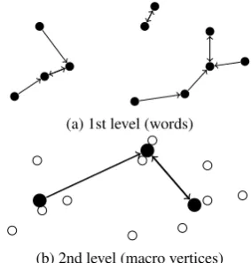
the relationship between different clusters is com-pletely lost. In order to deal with that, the sim-ple NNG can be extended via aneighborhood hi-erarchy (NH), which adds information about the neighborhood relation between clusters, clusters of cluster and so on. A sketch of the first two lev-els of such a hierarchy is given in fig.3. Each clus-ter is equipped with what could be called amacro vertex, which might for example be the mean of the vertices in the cluster, the center of the cluster root, or the most frequent (and thus hopefully most important) word in the cluster. Then the NNG of the macro vertices can be determined. This leads to new clusters, new macro vertices, another NNG and so forth, till the top level is reached, which contains only one cluster of macro vertices. In or-der to make the whole hierarchy browsable, the macro vertices can be given a clearer meaning by assigning one representative word to each of them. This word might for example be the nearest one to the macro vertex or the most frequent word in the cluster.
While the nearest neighbor relationship alone is somewhat problematic, as small changes in the dataset may result in huge differences in the cluster layout (in particular in high-dimensional spaces), the hierarchy smooths this effect away to some degree, as lower-level flipping between clus-ters will probably not affect higher level clusclus-ters.
(a) 1st level (words)
[image:3.595.343.485.466.615.2](b) 2nd level (macro vertices)
Figure 3: Sketch of a cluster hierarchy. The mas-sive dots are the centers of mass of the clusters of small dots and form a cluster themselves.
way paraphrasing terms for the words in their clus-ter (see section6 for semantic evaluation), under the given premise that similar words are mapped to nearby vectors. The NH produces a partitioning of the vector space in the spirit of a Voronoi dia-gram at various levels of coarseness and can thus be used to navigate through the otherwise hard to grasp high-dimensional space.
5.1 General Properties of the Hierarchy
The NH of theword2vecdataset has a total of six levels. The first level contains the words them-selves, higher levels comprise macro vertices as described above. General properties of the graphs on the different levels are given in table1. In ac-cordance with the hierarchical structure, the num-ber of words and thus the numnum-ber of clusters de-crease exponentially.
Typical characteristics of the graphs are strongly influenced by the fact that the graphs are NNGs. As each cluster has one root and each of thenvertices has out-degree one, thereciprocity
r:= #reciprocal edgesn (2)
is proportional to the inverse of the average num-ber of words per cluster. The more elaborate mea-sure of reciprocity ρ introduced by Garlaschelli and Loffredo(2004) reduces to
ρ= r(nn−−1)2−1 ≈
n1r (3)
and is thus almost the same as r for the larger graphs. Note that the expression (3) is not defined for the sixth level. ρ is rather low compared to other natural networks, but interestingly it lies just in the range of other word networks (Garlaschelli and Loffredo,2004).
Here, the depth d of the graphs for a specific leaf is the number of edges between the leaf and the respective cluster root. The average ofdover all leafs and the maximum value ofdare presented in table1. Whilemax(d)decreases exponentially, possibly in accordance with the shrinking of the cluster size, particularly the constancy of the mid-level∅dis striking and a sign of two contrary pro-cesses. The longer connections on the lower levels are compensated for by more small connections, or, in other words, the smaller high-level clusters are more regular in terms of their depths.
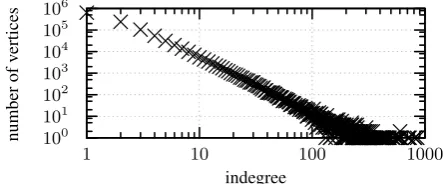
On all levels, the NNGs appear to be scale free (Barab´asi and Bonabeau,2003), with the
con-100 101 102 103 104 105 106
1 10 100 1000
number
of
vertices
indegree
Figure 4: Log-log scatter plot of the number of times a first-level vertex has a particular indegree. While this point cannot be represented in the chart, there are about1.8×106vertices with an indegree of 0 in the NNG.
level 1 2 3 4 5 6
# words 3·106 99,884 6750 540 55 2 # clusters 99,884 6750 540 55 2 1 ∅w./cl. 30.0 14.8 12.5 9.8 27.5 2.0 r 0.067 0.14 0.16 0.20 0.073 1.0 ρ 0.067 0.14 0.16 0.20 0.055 – ∅d 6.6 2.5 2.5 2.5 2.4 –
max(d) 25 16 10 6 4 –
Table 1: General properties of the NH of the
word2vec dataset. In the third row, the aver-age number of words per cluster is given. See sec-tion5.1for definitions of the other quantities.
straint that the higher-level graphs contain too lit-tle vertices for making a definite statement about that. Exemplarily, this feature can be seen for the first-level graph in fig. 4. Scale freeness is pri-marily associated to processes in which new tices are attached preferably to those existing ver-tices that already have a large indegree. In the current context this sheds a light on the behav-ior of the learning algorithm, specifically because scale freeness is encountered on all levels. A pos-sible interpretation is that the algorithm leads to a multi-level attaching of words and groups of words while trying to put similar words as close to each other as possible. Interestingly, different semantic networks exhibit the scale-free property, too (Steyvers and Tenenbaum,2005).
5.2 Examples of Clusters
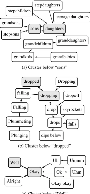
Examples of first-level clusters extracted from the
word2vecdataset can be found in fig.5. At this point, only the surface can be scratched, because there are thousands of such clusters and many of them are interesting in some way.
[image:4.595.308.530.68.160.2]sons grandsons
stepsons daughters stepchildren
granddaughters grandchildren
grandkids grandbabies stepdaughters
teenage daughters
(a) Cluster below “sons”
dropped
dropping falling
Falling
Plummeting
Plunging
drop
drops
skyrockets
falls dips below
dropoff Dropping
(b) Cluster below “dropped”
Well
Okay
Uh Ummm
Ok Uhm
Okay okay Alright
[image:5.595.95.269.62.437.2](c) Cluster below “Well”
Figure 5: Example clusters from actual dataset, with cluster roots marked gray. The most frequent word of the cluster is chosen as the macro vertex and given in the description.
proper names, capitalized or inflected words, mis-spellings, or fillers have not been stripped from the data. From the context-based training method (Mikolov et al.,2013) it can be expected that syn-tactically similar words end up close to each other, which is indeed seen in the NH, as in fig.5c, where fillers and certain discourse items, all of them cap-italized, form a cluster. This might also explain that only plural forms have gathered in fig. 5a. While this often means that connected items are also semantically similar, antonyms like “drops” and “skyrockets” in fig. 5b are frequently close to each other due to their similar syntactic roles. Despite such problems, it must be stressed that fig.5is not the result of extensive cherry picking, but that semantically meaningful clusters are the rule, even if the large number of proper names and
more or less meaningless padding words some-times shadow the more interesting clusters.
After this glance at some first-level clusters, an example of the actual hierarchy is shown in fig.6. On the lowest levels, the words are closely related to their neighbors and the words in their parent clusters, just as it has been the case in fig.5. This is still the case on the next levels, but, in general, the higher one gets in the hierarchy, the looser the connection to the words on the lower levels, be-cause a lot of words are collected beneath a spe-cific high-level word and not all of them can be equally suitable. In the specific situation in fig.6, the words on the third level are mostly related to fi-nance and economy and the same accounts for the fourth level, with more and more rather unspecific words in between. Revealing this is just what the hierarchy is good for: The fact that “index”-related words are collected in the “financial region” of the embedding space is not self-evident. If the em-beddings would not have been trained on a news corpus but on scientific resources, the position of the word “index” would very likely be a different one.
Here, the primary purpose of the NH is getting a better understanding of embeddings and the mean-ing of the relations in the NH must therefore not be over-interpreted, because they explicitly have to be left as unaltered as possible for making them good representatives of the raw dataset. Specific relations can often (see below) but not necessar-ily be transferred into a semantic order, as can ex-emplarily be seen in fig. 5a, where kinship rela-tions are not organized as one would probably put them. However, this is what the dataset looks like in terms of geometrical neighborhood. If certain words are positioned in a different way from what could be expected, this does not mean that the clustering went wrong, but rather that something interesting happened in the embedding space.
5.3 Geometry of Clusters
The neighborhood relation gives a good view of the relative positioning of the words, but the ge-ometry of the clusters and their orientation in the vector space is mostly veiled. Luckily, certain statistics reveal that there is much regularity in the shape of the clusters, so that the cluster alone con-tains enough information for telling where a spe-cific word is likely to be found.
ISECU.T
index
Dow Jones Stoxx Ifo
... ...
index indexes
index
composite index
Index
Composite Index Price Index
indexes indices
benchmark indices Indices Indexes 1st
le
vel
2nd
le
vel
3rd
le
[image:6.595.92.503.61.233.2]vel
Figure 6: Example of relations between clusters on the three lowest levels of the hierarchy. The dashed boxes frame clusters. Note that only an excerpt of the (much larger) cluster on the third level is shown. Lines ending in a circle indicate the connection between macro vertices and their clusters.
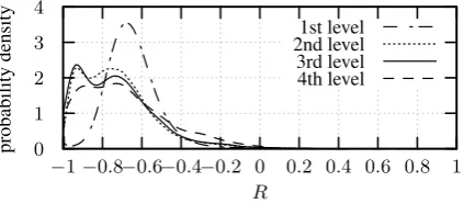
respective nearest neighbor w, the radiality R ∈ [−1,1]of this nearest neighbor relation can be de-fined as the normalized scalar product betweenv and the difference vector betweenwandvvia
R:= v|v·||(ww−−vv|). (4)
Positive values ofRmean, thatwlies farther away from the origin thanv, while negative values im-ply the opposite. In fig.7, the probability density for finding a certain value forRis shown. It can be
0 1 2 3 4
−1−0.8−0.6−0.4−0.2 0 0.2 0.4 0.6 0.8 1
probability
density
R
1st level 2nd level 3rd level 4th level
Figure 7: RadialityR, as defined in (4).
concluded that for the data at hand, the neighbor-hood relation on all levels strongly tends to point “inward”, i.e. towards the origin of the embedding space. In other words, it is almost certain, that the nearest neighbor of a word vector lies closer to the origin of the coordinate system than the word vec-tor itself. On this basis and as the clusters are ba-sically trees that grow away from the cluster root, it can be expected that the cluster roots typically lie near to the origin, compared to the other ver-tices in the respective cluster. This can be checked by plotting the probability density for finding a
cluster with a given percentage of vertices that are farther away from the origin than the cluster root (Figure8). As expected, in most clusters the
ma-0 1 2 3 4 5
0 0.2 0.4 0.6 0.8 1
probability
density
percentage of vertices 1st level
[image:6.595.310.524.362.453.2]2nd level 3rd level 4th level
Figure 8: Probability density for finding clusters where the given percentage of vertices lie farther away from the origin than the cluster root.
jority of vertices tends to lie farther outside than the cluster root. Nevertheless, the probability den-sity shows little bumps around fractions of small integers like 1
3, 12, or 23. These are mostly due to small clusters, for which the position of the cluster root within the cluster seems to be less predictable. However, these clusters contain only a small frac-tion of all words and their structure is easy to understand anyway. If only relatively large clus-ters are taken into account, the probability density peaks much more strongly around the value 1.
[image:6.595.77.289.473.566.2]“Falling”, “Plummeting”, and “Plunging” have an increasing L2-norm or distance from the origin and they form a chain in the graph in fig.5b. Only a bit additional information about the position of the root is thus sufficient for getting an idea of the position and orientation of the whole cluster.
6 Evaluation
The focus of this paper is on the analysis of em-beddings. Nevertheless, as already mentioned above, the findings presented in the previous sec-tions indicate that the NH might be used for NLP tasks beyond visualization of word embeddings or other large high-dimensional datasets, because the neighborhood and macro vertex relations appear to be connected to semantical relations between the words, particularly on the lower levels. Pos-sible tasks that directly come to mind are mea-suring relatedness or similarity, various kinds of tagging, and classification. In contrast to typi-cal semantitypi-cal frameworks like WordNet (Miller, 1995) or FrameNet (Baker et al., 1998) whose creation requires extensive human resources, the NH can be created without expert knowledge in a very short time and has the capability of including much more words.
Zesch and Gurevych(2007) analyze graphs ex-tracted from Wikipedia3and summarize a variety
of methods for evaluating semantical relations. In this spirit and for a first and quick quantitative view at the NH, similarity between neighbors in the graph and between words and their macro ver-tex are tested by calculating the respective Wu-Palmer similarity scores (Wu and Wu-Palmer, 1994) on WordNet (Miller, 1995). Other scores basi-cally lead to similar results and are thus not dis-cussed in more detail. Because the number of words inWordNetis much smaller than that in the dataset under consideration, the analysis is limited to those words that can be found in both datasets, which amounts to 54,586 words. For that to be possible, a NH of these words alone is used, which is distinct from the full hierarchy discussed above. The usefulness of these results for a much smaller dataset can be justified by envisioning that the sparser NNG must roughly be a skeleton of the full graph for geometrical reasons and must thus be related to the latter. Besides that, quantifying similarity on the smaller graph is interesting in its own right.
3http://www.wikipedia.org
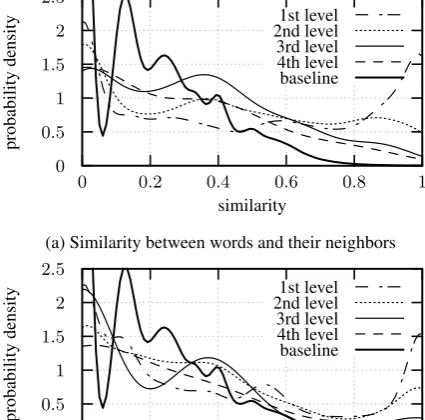
The results for the first four levels of the NH are shown in fig.9. Intuitively, the semantic rela-tions between neighbors or words and macro ver-tices are expected to be stronger, if more “proba-bility mass” can be found on the right side of the plot, because then more relations correspond to a higher similarity. In order to clarify the meaning of the curves, a baseline curve is added that corre-sponds to an equivalent evaluation of random word pairs.
Both the neighborhood relation and the macro vertex assignment yield noticeably better results than the baseline. In accordance with earlier re-marks, the curves confirm that the semantical sig-nificance of the hierarchy is much higher on the lower levels. While the first and the second level appear to exhibit a large amount of meaningful re-lations, the higher levels are not much better than the baseline.
0 0.5 1 1.5 2 2.5
0 0.2 0.4 0.6 0.8 1
probability
density
similarity 1st level 2nd level 3rd level 4th level baseline
(a) Similarity between words and their neighbors
0 0.5 1 1.5 2 2.5
0 0.2 0.4 0.6 0.8 1
probability
density
similarity 1st level 2nd level 3rd level 4th level baseline
[image:7.595.312.525.338.548.2](b) Similarity between words and their macro vertices Figure 9: Evaluation of similarity. The curves represent the probability density of finding a cer-tain Wu-Palmer similarity between the respective words. The baseline peaks at (0,6.8) but is cut off for clarity of the other curves.
7 Conclusion and Outlook
hier-archy (NH), a parameter free, flexible and gen-eral concept for clustering data in arbitrary spaces, which eliminates the problem of interpreting high-dimensional vectors while preserving the most im-portant geometric information. In order to get a better understanding of the data, a variety of sta-tistical properties of word embeddings has been evaluated. First evidence of the semantic signifi-cance of the NH has been established by relating it to WordNet data.
This method of analysis will allow researchers to interactively explore the neighborhood relations in an embedding space. This will enable them not only to get a better intuition of the structure of em-bedding spaces but will also give them new ideas on how to incorporate embeddings in natural lan-guage processing tasks like information extraction or other tasks that require semantic knowledge. Acknowledgments
This work was funded by the Deutsche Forschungsgemeinschaft (DFG) under grant SFB 1102.
References
Collin F. Baker, Charles J. Fillmore, and John B. Lowe. 1998. The Berkeley FrameNet Project. In Pro-ceedings of the 36th Annual Meeting of the Asso-ciation for Computational Linguistics and 17th In-ternational Conference on Computational Linguis-tics, Volume 1. Association for Computational Lin-guistics, Montreal, Quebec, Canada, pages 86–90. https://doi.org/10.3115/980845.980860.
Albert-L´aszl´o Barab´asi and Eric Bonabeau. 2003. Scale-free networks. Scientific American
288(5):60–69. https://doi.org/10.1038/scientifi-camerican0503-60.
Marco Baroni, Georgiana Dinu, and Germ´an Kruszewski. 2014. Don’t count, predict! A systematic comparison of context-counting vs. context-predicting semantic vectors. InProceedings of the 52nd Annual Meeting of the Association for Computational Linguistics (Volume 1: Long Papers). Association for Computational Lin-guistics, Baltimore, Maryland, pages 238–247. http://www.aclweb.org/anthology/P14-1023. Ciprian Chelba, Tomas Mikolov, Mike Schuster,
Qi Ge, Thorsten Brants, and Phillipp Koehn. 2013. One Billion Word Benchmark for Measuring Progress in Statistical Language Modeling. CoRR
abs/1312.3005. http://arxiv.org/abs/1312.3005. Diego Garlaschelli and Maria I. Loffredo. 2004.
Patterns of Link Reciprocity in Directed
Networks. Physical Review Letters 93(26). https://doi.org/10.1103/physrevlett.93.268701.
Tatsunori Hashimoto, David Alvarez-Melis, and Tommi Jaakkola. 2016. Word Embeddings as Metric Recovery in Semantic Spaces. Transac-tions of the Association for Computational Lin-guistics 4:273–286. https://transacl.org/ojs/in-dex.php/tacl/article/view/809.
Anil K. Jain, M. Narasimha Murty, and Patrick J. Flynn. 1999. Data Clustering: A Review.
ACM computing surveys (CSUR) 31(3):264–323. https://doi.org/10.1145/331499.331504.
Omer Levy, Yoav Goldberg, and Ido Dagan. 2015. Improving distributional similarity with lessons learned from word embeddings. Trans-actions of the Association for Computational Linguistics 3:211–225. https://transacl.org/ojs/in-dex.php/tacl/article/view/570.
Laurens van der Maaten and Geoffrey Hinton. 2008. Visualizing data using t-SNE. Journal of Machine Learning Research9(Nov):2579–2605.
Tomas Mikolov, Ilya Sutskever, Kai Chen, Greg S Cor-rado, and Jeff Dean. 2013. Distributed representa-tions of words and phrases and their compositional-ity. InAdvances in Neural Information Processing Systems. pages 3111–3119.
George A. Miller. 1995. WordNet: A Lexical Database for English. Com-munications of the ACM 38(11):39–41. https://doi.org/10.1145/219717.219748.
Marius Muja and David G. Lowe. 2009. Fast approx-imate nearest neighbors with automatic algorithm configuration. Proceedings of the Conference on Computer Vision Theory and Applications (VISAPP) (1)2(331-340):2.https://doi.org/10.1.1.160.1721.
Sascha Rothe and Hinrich Sch¨utze. 2016. Word Em-bedding Calculus in Meaningful Ultradense Sub-spaces. In Proceedings of the 54th Annual Meet-ing of the Association for Computational LMeet-inguistics (Volume 2: Short Papers). Association for Computa-tional Linguistics, Berlin, Germany, pages 512–517. http://anthology.aclweb.org/P16-2083.
Jagan Sankaranarayanan, Hanan Samet, and Amitabh Varshney. 2007. A fast all nearest neighbor algorithm for applications involving large point-clouds. Computers & Graphics 31(2):157–174. https://doi.org/10.1016/j.cag.2006.11.011.
Tobias Schnabel, Igor Labutov, David Mimno, and Thorsten Joachims. 2015. Evaluation methods for unsupervised word embeddings. InProceedings of the 2015 Conference on Empirical Methods in Natu-ral Language Processing. Association for Computa-tional Linguistics, Lisbon, Portugal, pages 298–307. http://aclweb.org/anthology/D15-1036.
Mark Steyvers and Joshua B. Tenenbaum. 2005. The Large-scale structure of semantic networks: Statisti-cal analyses and a model of semantic growth. Cog-nitive Science29(1):41–78.
Antoine Tixier, Konstantinos Skianis, and Michalis Vazirgiannis. 2016. GoWvis: A Web Applica-tion for Graph-of-Words-based Text VisualizaApplica-tion and Summarization. In Proceedings of ACL-2016 System Demonstrations. Association for Computa-tional Linguistics, Berlin, Germany, pages 151–156. http://anthology.aclweb.org/P16-4026.
Laurens Van Der Maaten, Eric Postma, and Jaap Van den Herik. 2009. Dimensionality Reduction: A Comparative Review. Journal of Machine Learning Research10:66–71.
Zhibiao Wu and Martha Palmer. 1994. Verb Seman-tics and Lexical Selection. In Proceedings of the 32nd Annual Meeting of the Association for Compu-tational Linguistics. Association for Computational Linguistics, Las Cruces, New Mexico, USA, pages 133–138. https://doi.org/10.3115/981732.981751. Yadollah Yaghoobzadeh and Hinrich Sch¨utze. 2016.
Intrinsic Subspace Evaluation of Word Embedding Representations. InProceedings of the 54th Annual Meeting of the Association for Computational Lin-guistics (Volume 1: Long Papers). Association for Computational Linguistics, Berlin, Germany, pages 236–246. http://www.aclweb.org/anthology/P16-1023.