Phase space equilibrium distributions and their applications to spin systems with nonaxially symmetric Hamiltonians

Phase-space equilibrium distributions and their applications to spin systems with nonaxially

symmetric Hamiltonians

Yuri P. Kalmykov,1 William T. Coffey,2and Serguey V. Titov2,3

1_{Laboratoire de Mathématiques, Physique et Systèmes, Université de Perpignan, 52, Avenue de Paul Alduy,}

66860 Perpignan Cedex, France

2_{Department of Electronic and Electrical Engineering, Trinity College, Dublin 2, Ireland}

3_{Institute of Radio Engineering and Electronics, Russian Academy of Sciences, Vvedenskii Square 1, Fryazino 141190, Russia}

共Received 29 November 2007; revised manuscript received 31 January 2008; published 13 March 2008兲 The Fourier series representation of the equilibrium quasiprobability density functionW_S共␽,␸兲 or Wigner function of spin “orientations” for arbitrary spin Hamiltonians in a representation共phase兲space of the polar angles共␽,␸兲 共analogous to the Wigner function for translational motion兲arising from the generalized coherent state representation of the density operator is evaluated explicitly for some nonaxially symmetric problems including a uniaxial paramagnet in a transverse external field, a biaxial, and a cubic system. It is shown by generalizing transition state theory to spins 关i.e., calculating the escape rate using the equilibrium density functionWS共␽,␸兲only兴that one may evaluate the reversal time of the magnetization. The quantum corrections to the transition state theory escape rate equation for classical magnetic dipoles appearbothin theprefactor

and in theexponential partof the escape rate and exhibit a marked dependence on the spin number. Further-more, the phase-space representation allows us to estimate the switching field curves and/or surfaces for spin systems because quantum effects in these fields can be estimated via Thiaville’s geometrical method关Phys. Rev. B 61, 12221共2000兲兴for the study of the magnetization reversal of single-domain ferromagnetic particles. The calculation is accomplished共just as the determination of the equilibrium quasiprobability distributions in the phase space of the polar angles兲 by calculating switching field curves and/or surfaces using the Weyl symbol共c-number representation兲 of the Hamiltonian operator for given magnetocrystalline-Zeeman energy terms. Examples of such calculations for various spin systems are presented. Moreover, the reversal time of the magnetization allows us to estimate thermal effects on the switching fields for spin systems.

DOI:10.1103/PhysRevB.77.104418 PACS number共s兲: 75.45.⫹j, 75.40.Gb, 75.50.Tt, 75.50.Xx

I. INTRODUCTION

The interpretation of spin relaxation experiments com-prises a fundamental problem of condensed phase physics and chemistry yielding a well defined means of extracting information concerning the structure and characteristics of materials as a function of spin S so providing a bridge be-tween microscopic and macroscopic physics. For example 共recalling that the number of spins in a sample roughly cor-responds to the number of atoms兲, on an atomic level, nuclear magnetic and related spin resonance experiments, etc., examine the time evolution of the individualelementary spins1,2 _{of nuclei, electrons, muons, etc., while on} mesos-calesthe time evolution of magneticmolecular clusters共i.e., spins 15– 25␮B兲exhibiting relatively large quantum effects is

currently of interest in the fabrication of molecular magnets.3

On nanoscalessingle-domain ferromagnetic particles共giant

spins 104_{– 10}5_␮

B兲 with a given orientation of the particle

moment and permanent magnetization exist. These have spawned very extensive magnetic recording industries, the particles commonly used being on or near the microsize scale. Finally, on thebulk macroscopic scaleone has perma-nent magnets 共1020_␮

B兲, i.e., multidomain systems where

magnetization reversal occurs via themacroscopicprocesses of nucleation, propagation and annihilation of domain walls. Thus a well defined size scale ranging from the bulk macro-scopic down to individual atom and spins naturally exists.

On an atomic level spin relaxation experiments in nuclear magnetic or electron spin resonance are usually interpreted

via the phenomenological Bloch4_{equations pertaining to the} relaxation of elementary spins subjected to an external mag-netic field and interacting with an environment that is as-sumed to be a heat reservoir at constant temperature T. On mesoscales both the behavior of the hysteresis loop and the relaxation or reversal time of the magnetization as a function of S are of extreme importance in the observation of the transition from microscopic to nanoscale physics as strong quantum effects are likely to occur as the spin decreases corresponding to the transition from a behavior reminiscent of a single-domain ferromagnetic nanoparticle to that of a molecular cluster. In this region the magnetization may re-verse by resonant quantum tunneling as may be observed in the corresponding hysteresis loop.5_{In contrast on the} nanos-cale in single-domain ferromagnetic nanoparticles共originally encountered in paleomagnetism in the context of past rever-sals of Earth’s magnetic field, where depending on the size of the particle, the relaxation time may vary from milliseconds to millions of years兲the relaxation is treated as classical and proceeds by uniform rotation as conjectured by Néel6 _and Stoner and Wohlfarth.7_{The relaxation time epochs} represent-ing the transition from giant Langevin paramagnetic behav-ior共superparamagnetism兲with no hysteresis involved via the magnetic after effect stage 共where the relaxation time for changes in orientation of the magnetization is of the order of the time of a measurement兲to stable ferromagnetism where a given ferromagnetic state corresponds to one of many pos-sible such metastable states in which the magnetization vec-tor is held in a preferred orientation. In the hypothesis of

uniform or coherent rotation the exchange energy which is supposed constant renders all spins collinear and the magni-tude of the magnetization vector is constant in space hence competition exists only between the anisotropy energy and the Zeeman energy of the applied field since the magnetiza-tion vector is perfectly aligned. This hypothesis should hold for small sample sizes, i.e., single-domain particles, where domain walls cannot form in the sample共i.e., it is energeti-cally unfavorable to form them兲and at high fields in samples of low coercivity.8

As far as dynamics are concerned, Néel6 _{determined the} magnetization relaxation time, i.e., the time of reversal of the magnetization of the particle, due to thermal agitation over its internal magnetocrystalline anisotropy barrier from the inverse escape rate over the barriers using transition state theory共TST兲9_{as specialized to magnetic moments. Thus his} treatment given in detail for uniaxial anisotropy only is con-fined to a discrete set of orientations for the magnetic mo-ment of the particle. Moreover, the equilibrium distribution is all that is ever required since the disturbance to the Bolt-zmann distribution in the wells of the magnetocrystalline an-isotropy potential due to the escape of the magnetization over the barrier is ignored. In addition the effect of an exter-nal applied field 共Zeeman energy term兲 can be included which is important because5 _{at low temperatures with zero} applied field the energy barrier between two states of oppo-site magnetization is much too high for thermally agitated escape to occur. The barrier height, however, may be reduced by applying an external共biasing兲field in the opposite direc-tion to that of the magnetizadirec-tion of the particle. If the exter-nal field iscloseto the switching field atzero temperature共at which the magnetization reverses兲 thermal fluctuations are then strong enough to overcome the anisotropy-Zeeman en-ergy barrier hence the magnetization is reversed.

The static magnetization currents of single-domain par-ticles are usually calculated using the method of Stoner and Wohlfarth.7 _{Their procedure simply consists in minimizing} the free energy of the particle comprising the sum of Zeeman and anisotropy energies with respect to the polar and azi-muthal angles specifying the orientation of the magnetization for each value of the applied field. The calculation always leads to hysteresis because in certain field ranges10,11_{two or} more minima exist and thermally agitated transitions be-tween them are neglected. The value of the applied field, at which the magnetization reverses, is as we saw above called the switching field and the angular dependence of that field with respect to the easy axis of the magnetization yields the well known Stoner–Wohlfarth astroids.7 _{These were} origi-nally given for uniaxial shape anisotropy only which is the anisotropy of the magnetostatic energy of the sample induced by its nonspherical shape. The astroids represent a paramet-ric plot of the parallel versus the perpendicular component of the switching field which in the uniaxial case is the field that destroys the bistable structure of the free energy. The astroid concept was later generalized to arbitrary effective aniso-tropy by Thiaville8 _{including any given magnetocrystalline} anisotropy and even surface anisotropy. He proposed a geo-metrical method for the calculation of the energy of a particle allowing one to determine the switching field for all values of the applied magnetic field yielding the critical switching

field surface analogous to the Stoner–Wohlfarth astroids. A knowledge5 of the switching field surface allows one to de-termine the effective anisotropy of the particle and all other parameters such as the frequencies of oscillations in the wells of the potential, i.e., the ferromagnetic resonance fre-quency, etc. We reiterate that these static calculations all ig-nore thermal effects on the switching field, i.e., transitions between the minima of the potential are neglected so that they are strictly only valid at zero temperature.

In the context of thermal effects giving rise to transitions between the potential minima we have mentioned that the original dynamical calculations of Néel for single-domain particles utilize classical transition state theory. In the more recent treatment formulated by Brown10,11 _{共now known as} the Néel–Brown model兲,5 _{which explicitly treats the system} as a gyromagnetic one and which includes nonequilibrium effects due to the loss of magnetization at the barrier, the time evolution of the magnetization of the particleM共t兲 is described by a classical Langevin equation. This is the phe-nomenological Landau–Lifshitz12 or Gilbert equation13,14 originally used to study the motion of a domain wall aug-mented by torques due to random white noise magnetic fields characterizing the giant spin-bath interaction. In the absence of damping and stochastic terms this equation corresponds to the Larmor equation for the motion of the giant spin so in-cluding the gyromagnetic effects. The Langevin equation of motion of the magnetization 共which inter alia reconciles Néel’s treatment of magnetization reversal with the general theory of the Brownian motion15_{and allows for a continuous} distribution of the magnetic moment orientations兲yields10,11 the Fokker–Planck equation for the surface distribution of the magnetic moment orientations on the unit sphere. More-over, the reversal time may be asymptotically calculated共in the high barrier limit as the relaxation time is of the order of the time of measurement in an experiment兲by means of the Kramers escape rate theory9,16,17_{as adapted to magnetic} mo-ments by Brown.10,11 _{The resulting asymptotic expressions} may then be compared with the exact results for the reversal time yielded by the inverse of the smallest nonvanishing ei-genvalue of the Fokker–Planck equation which may be ex-tracted from the solution of that equation by matrix contin-ued fraction methods as has been accomplished in Refs.15 and18 for many anisotropy potentials. The asymptotic ex-pressions are valid in various dissipation regimes delineated by the ratio of the magnetization energy lost per cycle of the almost periodic motion of the magnetization at the lowest saddle point energy of the potential to the thermal energy.17 Moreover, thermal effects on the switching field astroids due to transitions between the minima of the potential may be calculated by equating the inverse escape rate to the measur-ing time in a given experiment and solvmeasur-ing the resultmeasur-ing implicit equation for the switching field numerically, com-prising a classical treatment of the hysteresis loop at nonzero temperatures.

Now Bean and Livingston19 _{have suggested that in a} single-domain particle besides the overbarrier Néel process the magnetization may also reverse bymacroscopic quantum

tunneling 共macroscopic since a giant spin is involved兲

size and the temperature and spin dependence of the associ-ated Stoner–Wohlfarth hysteresis loops and astroids must be studied in order to distinguish tunneling reversal from rever-sal by thermal agitation. Thus systematic ways of introduc-ing quantum effects into the magnetization reversal of a na-nomesoscale particle 共which in general may be restated as quantum effects in parameters characterizing the decay of metastable states in spin systems兲are required. In general the magnetization may reverse by quantum tunneling for rela-tively smallSor at very low temperatures for largerSwhich may be observed in the behavior of the Stoner–Wohlfarth asteroids. In general, so important are quantum effects in the magnetization reversal in spin systems that diverse theoreti-cal methods, e.g., WKB formalism,20 _{instantons; mapping} of the spin Hamiltonian onto equivalent particle Hamiltonians;21,22 _{perturbation treatment of} quantum-classical escape rate transitions;23 _{etc., have been developed} in order to treat them. Yet another approach 共that adopted here兲is the extension of Wigner’s phase-space representation of the density operator24,25 _{共originally developed to obtain} quantum corrections to the classical distributions for point particles in the phase space of positions and momenta兲to the description of spin systems共see, e.g., Refs.26–33兲.

The phase-space共or generalized coherent state兲 represen-tation of the spin density matrix allows one to describe spin systems in terms of a quasiprobability density function or Wigner functionWS共␽,␸兲 of spin orientations in the phase

共here configuration兲space共␽,␸兲;␽and␸are the polar and azimuthal angles, respectively, constituting the canonical variables. The advantage of such a mapping of the density matrix onto a c-number quasiprobability density function WS共␽,␸兲 as extensively used in quantum optics 共see, e.g.,

Ref.25兲is that it is possible to show howWS共␽,␸兲evolves

as a function of the spin sizeS. In the limit of large spins, WS共␽,␸兲 reduces to the classical Boltzmann orientational

distribution naturally linking the equilibrium quantum and classical spin regimes. The quasiprobability densityWS共␽,␸兲

was originally introduced by Stratonovich31_{as part of a} gen-eral discussion ofc-number quasiprobability distributions for quantum systems in a representation space based on the sym-metry properties of the underlying group. Examples are the Heisenberg–Weyl group for particles and the SU共2兲 group for rotations.

Agarwal and co-workers34,35 _{have explicitly given the} phase-space distributions for atomic angular momentum Dicke states, coherent states, and squeezed states corre-sponding to a collection of two-level atoms. In the magnetic context, explicit equations for the equilibrium distributions WS共␽,␸兲have been obtained for an assembly of spinsSin a

uniform magnetic fieldH共Refs.26and33兲and spins in the simplest uniaxial potential of the magnetocrystalline aniso-tropy and Zeeman energy.36Moreover, the results have been used37 _{to generalize Néel’s classical calculation of} magneti-zation escape rates to include spin size effects for the sim-plest uniaxial potential in a uniform external magnetic field applied parallel to the anisotropy axis using quantum transi-tion state theory as adopted to spins in the manner pioneered by Wigner38 _{for point particles. However, because of the} limitation to axially symmetric potentials 共e.g., one cannot

treat surface anisotropy energy, magnetoelastic anisotropy energy, etc.兲 these calculations comprise a very restricted treatment of spin size effects. The first step toward a general treatment of these in the magnetic context is to calculate the equilibrium phase-space distribution function WS共␽,␸兲as a

function of spin size for givennonaxially symmetric effective

anisotropy-Zeeman energy Hamiltonians which is one

pur-pose of this paper. Having determined the various equilib-rium distributions corresponding to particular anisotropies, our second purpose is to calculate the Stoner–Wohlfarth magnetization curves represented in switching field astroid form as a function of spin size for nonaxially symmetric potentials. This calculation generalizes Thiaville’s8 geometri-cal method共for the construction of switching field curves for such potentials兲to include quantum effects due to finite spin size permitting one to study the behavior of the astroids in the interesting magnetic cluster—single-domain particle transition region. Finally, we estimate the reversal time of the magnetization via the quantum generalization of TST 共previ-ously elaborated for the axially symmetric uniaxial potential兲.37_{This will allow one to estimate temperature} ef-fects in the astroids and hysteresis loops within the limita-tions imposed by quantum TST共moderate damping, etc.兲.39

Our calculation proceeds, by generalizing the axially sym-metric results described in Ref. 36 pertaining to a spin S where the external uniform fieldH is parallel to the aniso-tropy axis, to show how phase-space distributions of spins can be obtained both analytically and numerically for various

nonaxially symmetric spin systems with equilibrium states

described by a canonical density matrix␳ˆ given by

␳ˆ=e−␤HˆS/_Z

S. 共1兲

HereZS= Tr兵e−␤H ˆ

S其_{is the partition function for a spin system}

with an arbitrary nonaxially symmetric HamiltonianHˆSand

␤= 1/共kT兲 is the inverse thermal energy. We shall at first illustrate the analytical method by evaluatingWS共␽,␸兲for an

assembly of noninteracting spins 共essentially5 _that corre-sponding to the quantum treatment of superparamagnetism so that in the absence of a field the spins are randomly ori-ented兲 in an externalconstantfield Hwith an arbitrary di-rection in space so that the Hamiltonian of a spin is

␤HˆS= −␤␥បH·Sˆ = −␰共␥XSˆX+␥YSˆY+␥ZSˆZ兲, 共2兲

where ␥X,␥Y,␥Z are the direction cosines of H, ␥ is the

gyromagnetic ratio, ប is Planck’s constant, and ␰is the di-mensionless external field parameter. Next we consider vari-ous magnetic anisotropies establishing one or more preferred orientations of the magnetization of an assembly of spins. In particular, we shall consider a uniaxial paramagnet in a trans-verse external field with

␤HˆS= −␰SˆX−␴SˆZ2. 共3兲

the quantum case will enhance the tunneling probability. Next we will consider biaxial- and cubic systems, with Hamiltonians

␤HˆS= −␴SˆZ2−␦共SˆX2−SˆY2兲 共4兲

and

␤HˆS= −␰SˆZ−␴共SˆX4+SˆY4+SˆZ4兲/2. 共5兲

Here ␦ and ␴ are dimensionless anisotropy barrier height parameters. For clarity we summarize the basic features of the Wigner–Stratonovich transformation of the density ma-trix. Equilibrium distribution functions for the particular Hamiltonians so determined may then be used to study the equilibrium magnetization, switching field hysteresis curves, etc., which require only a knowledge of these distributions.

II. WIGNER–STRATONOVICH TRANSFORMATION OF THE DENSITY MATRIX

The phase-space distribution function W_S共s兲共␽,␸兲 or Wigner function on the surface of the unit sphere for a spin system given by Stratonovich31共see also Refs.27and28兲is defined by the invertible map

WS共 s_兲共

␽,␸兲= Tr兵␳ˆ wˆs共␽,␸兲其, 共6兲

wheresparametrizes quasiprobability functions of spins be-longing to the SU共2兲dynamical symmetry group considered here; the Wigner–Stratonovich operator共or kernel兲wˆs共␽,␸兲

is defined as27,28

wˆs共␽,␸兲=

冑

4␲ 2S+ 1L

兺

=0

2S

兺

M=−L L

共CS,S,L,0

S,S _兲−s

Y_L*_,MTˆL共,M S兲

. 共7兲

Here the asterisk denotes the complex conjugate,YL,M共␽,␸兲

are the spherical harmonics,40Tˆ_L共S_,M兲 are the irreducible tensor 共polarization兲operators with matrix elements40

关TˆL共,M S_{兲 兴}

m⬘,m=

冑

2L+ 1 2S+ 1CS,m,L,M

S,m⬘

, 共8兲

and C_SS_,,_SS_,L,0 and CS_S,_,mm_,⬘_L,M are the Clebsch–Gordan coefficients.40 _{The density matrix ␳ˆ may then be expressed} using the kernel equation共7兲via the inverse transformation

␳ˆ=2S+ 1

4␲

冕

_␪,␸wˆs共␽,␸兲WS 共−s兲_共␽

,␸兲sin␽d␽d␸.

The functionW_S共−s兲共␽,␸兲now allows us to calculate the av-eragevalue具Aˆ典= Tr兵␳ˆ Aˆ其of an arbitrary spin operatorAˆ be-cause theW_S共−s兲共␽,␸兲 provide the overlap relation28

具Aˆ典=2S+ 1 4␲

冕

_␪,␸A

共s兲_共␽

,␸兲WS共

−s_兲共

␽,␸,t兲sin␽d␽d␸,

whereA共s兲_{共␽,␸兲= Tr兵Aˆ wˆ}

s共␽,␸兲其 is the Weyl symbol of the

operator Aˆ. The parameter values s= 0 and s=⫾1 corre-spond to the Stratonovich31 _{and Berezin}32 _{contravariant and}

covariant functions, respectively 共the latter are directly re-lated to the P and Q symbols appearing naturally in the coherent state representation; see Ref.27for a review兲. Here we considerW_S共−1兲共␽,␸兲only omitting everywhere the super-script −1 in W_S共−1兲共␽,␸兲 关W_S共1兲共␽,␸兲 and W_S共0兲共␽,␸兲 can be treated in like manner兴. We have chosenW_S共−1兲共␽,␸兲because it alone satisfies the non-negativity condition required of a true probability density function, viz., W共−1兲共␽,␸兲艌0. The quasiprobability densities W_S共1兲共␽,␸兲 andW_S共0兲共␽,␸兲 violate this condition 共they may take on negative values in the present problem兲. The relationship of the Wigner– Stratonovich operator wˆ₋₁共␽,␸兲 from Eq. 共7兲 to various equivalent forms26 _{of the generalized coherent state} repre-sentation of the density matrix is given in the Appendix.

The phase-space distribution may be presented for arbi-trarySin共finite兲Fourier series form共which emphasizes the relationship with the conventional infinite Fourier series rep-resentation of the associated classical Boltzmann distribution in terms of spherical harmonics兲, namely,

2S+ 1

4␲ WS共␽,␸兲=

兺

L=0 2S

兺

M=−L L

具YL,M典Y*L,M共␽,␸兲, 共9兲

where 具YL,M典=关共2S+ 1兲/4␲兴兰02␲兰0␲YL,M共␽,␸兲WS共␽,␸兲 ⫻sin␽d␽d␸are the equilibrium values of the spherical har-monics given explicitly by

具YL,M典=

冑

2S+ 1 4␲ CS,S,L,0

S,S

aL,M. 共10兲

Here the coefficientsaL,M共representing expectation values of

Tˆ_L共S_,M兲 in a state described by the density matrix␳ˆ兲are40

aL,M=具TˆL共,M S兲 _典

= Tr兵␳ˆ TˆL共,M S兲 _其

. 共11兲

Equation 共9兲 is a general result valid for an arbitrary spin system with equilibrium states described by the canonical density matrix ␳ˆ given by Eq. 共1兲 with an arbitrary model Hamiltonian HˆS共SˆX,SˆY,SˆZ兲 expressed in terms of the spin

operatorsSˆX, SˆY, and SˆZ. The spin operators can be written

using the polarization operatorsTˆ_1,共S_M兲 as40

SˆX=a关Tˆ1,−1共

S兲

−Tˆ_1,1共S兲兴, SˆY=ia关Tˆ1,−1共

S兲

+Tˆ_1,1共S兲兴, SˆZ=

冑

2aTˆ1,0共

S兲

, 共12兲 wherea=

冑

S共S+ 1兲共2S+ 1兲/6. Thus using Eqs.共8兲and共12兲, we can 共i兲 present the Hamiltonian HˆS in explicit matrix

form, next, 共ii兲 evaluate numerically the density matrix ␳ˆ from Eq. 共1兲, and then 共iii兲 calculate the coefficients aL,M

from Eq.共11兲and so the Fourier coefficients具YL,M典from Eq.

共10兲, having thus estimated具YL,M典, we can共iv兲calculate the

phase-space distributionWS共␽,␸兲from the finite Fourier

se-ries equation共9兲 for any particularS. Moreover, the results can be presented in closed form whenever the equilibrium spin density matrix ␳ˆ=e−␤HˆS/_Z

S or its elements are given

explicitly.

evalu-ate WS共␽,␸兲 for given S. However, for calculation of

par-ticular observables such as the magnetization only a few mo-ments may be necessary. For example, in the calculation of the longitudinal,具SˆZ典, and transverse,具SˆX典and具SˆY典,

compo-nents of the magnetization, noting the correspondence rules of operators SˆX, SˆY, SˆZ and Weyl symbols 共c numbers兲

SX共␽,␸兲, SY共␽,␸兲, SZ共␽,␸兲 in the phase space 共␽,␸兲,28

namely,

SˆX→SX=

冑

2␲S共S+ 1兲/3

兺

L=0 2S

兺

M=−L L

CS,S,L,0

S,S

Y_L*_,M

⫻Tr兵共Tˆ_1,−1共S兲 −Tˆ_1,1共S兲兲TˆL共,M S_{兲 其}

=

冑

2␲/3共S+ 1兲共Y1,−1+Y1,1兲,

SˆY→SY=i冑2␲S共S+ 1兲/3

兺

L=0 2S

兺

M=−L L

CS,S,L,0

S,S

Y_L*_,M

⫻Tr兵共Tˆ_1,−1共S兲 +Tˆ_1,1共S兲兲TˆL共,M S兲 _其

=i冑2␲/3共S+ 1兲共Y1,−1−Y1,1兲, and

SˆZ→SZ=

冑

4␲S共S+ 1兲/3

兺

L=0 2S

兺

M=−L L

CS,S,L,0

S,S

Y_L*_,MTr兵Tˆ_1,0共S兲TˆL共,M S兲 _其

=

冑

4␲/3共S+ 1兲Y1,0, we have

具SˆX典=

冑

2␲/3共S+ 1兲关具Y1,−1典+具Y1,1典兴, 共13兲

具SˆY典=i冑2␲/3共S+ 1兲关具Y1,−1典−具Y1,1典兴, 共14兲 and

具SˆZ典=

冑

4␲/3共S+ 1兲具Y1,0典. 共15兲 Here we have used the property of polarization operators40

Tr兵TˆL共₁,M₁ S_兲

TˆL共₂,M₂ S_{兲 其}

=共− 1兲M1␦

L₁,L₂␦M₁,−M₂. 共16兲

Thus only具Y_1,0典 and具Y_1,⫾1典 are now required.

The results obtained so far are entirely formal. Now we shall demonstrate how the phase-space distributions for par-ticular spin systems can be obtained for all S 共integer and half-integer兲.

III. SPIN IN A UNIFORM EXTERNAL FIELD

As the simplest example of the Fourier series method em-bodied in Eqs.共9兲and共10兲, we calculate the Wigner function of a spin in an external uniform field with Hamiltonian

␤HˆS= −␰共␥XSˆX+␥YSˆY+␥ZSˆZ兲,

which yields the conventional theory of superparamag-netism. Here the matrix elements of HˆS can be given in

closed form, viz.,

关HˆS兴m⬘,m=A共−兲␦m,m⬘+1+A共+兲␦m,m⬘−1−␥Z␰m␦m,m⬘

where A共⫾兲= −共1/2兲␰共␥X⫾i␥Y兲

冑

共S⫾m兲共S⫿m+ 1兲.

Further-more, for any particular S the density matrix ␳ˆS=e−␤H ˆ

S/_Z S

can be presented as a finite series of spin operators共using the commutation relations for spin operators兲.40_{For example, for} S=1₂,S= 1, etc., one has

␳ˆ_1/2= 1 Z1/2

关cosh共␰/2兲Iˆ+ 2 sinh共␰/2兲共␥XSˆX+␥YSˆY+␥ZSˆZ兲兴,

共17兲

␳ˆ₁= 1 Z1

关Iˆ+ sinh␰共␥XSˆX+␥YSˆY+␥ZSˆZ兲

+ 2 sinh2共␰/2兲共␥XSˆX+␥YSˆY+␥ZSˆZ兲2兴, 共18兲

etc., whereIˆis the identity matrix. The corresponding phase-space distributionWS共␽,␸兲 can then be calculated共after

te-dious matrix algebra best accomplished, e.g., via MATH-EMATICA兲 from Eqs. 共9兲–共12兲 using the properties of

polarization operators such as Eq.共16兲and40 Tr兵TˆL共₁,M₁

S兲

TˆL共₂,M₂ S兲

TˆL共₃,M₃ S兲 _其

=共− 1兲2S+L3+M3

冑

共2_L

1+ 1兲共2L2+ 1兲

⫻CL₁,M₁,L₂,M₂

L₃,−M₃

再

L1 L2 L3

S S S

冎

, 共19兲

where

兵

L1S S SL2L3

其

is a 6jsymbol.40The finite series can then be

summed so that the distributionWS共␽,␸兲 can be written in

closed form for arbitrary spin valuesS as

WS共␽,␸兲=关cosh共␰/2兲+ sinh共␰/2兲F共␽,␸兲兴2S/ZS, 共20兲

whereF共␽,␸兲=␥Xsin␽cos␸+␥Ysin␽sin␸+␥Zcos␽and

ZS=

2S+ 1 4␲

冕

₀

␲

冕

0

2␲

关cosh共␰/2兲

+ sinh共␰/2兲F共␽,␸兲兴2Ssin␽d␽d␸

= sinh关共S+ 1/2兲␰兴/sinh共␰/2兲 共21兲 is the partition function. For three particular cases

␥X= 1, ␥Y= 0, ␥Z= 0; ␥X= 0, ␥Y= 1,

␥Z= 0; and␥X= 0, ␥Y= 0, ␥Z= 1,

Eq. 共20兲 reduces to the known equations of Takahashi and Shibata.33 The average equilibrium magnetization of a spin, namely,MH=g␮B具Sˆ ·H典, is

MH=g␮B

共2S+ 1兲共S+ 1兲 4␲

⫻

冕

0 ␲

冕

0 2␲

F共␽,␸兲WS共␽,␸兲sin␽d␽d␸

where␮B is the Bohr magneton,g is the Landé factor, and

BS共x兲is the Brillouin function defined as27

BS共x兲=

2S+ 1 2S coth

冉

2S+ 1 2S x

冊

−

1 2S coth

冉

x

2S

冊

. 共23兲 In the classical limit,␤→0,S→⬁, and␤S= const, the equi-librium distribution WS共␽,␸兲 共which now becomes a

conventional Fourier series兲 and the Brillouin function BS共x兲 tend, respectively, to the Boltzmann distribution

共2S+ 1兲WS共␽,␸兲/4␲→Zcl−1eS␰F共␽,␸兲 and the Langevin

func-tion BS共x兲→L共x兲= coth共x兲− 1/x, where Zcl is the classical

partition function. This comprises the usual treatment of su-perparamagnetism, the only difference from the conventional theory of paramagnetism being that the magnetic moments of the particles are enormous. Quantum effects become im-portant when ␤ប␥H/S艌1, i.e., either at smallS or at very low temperaturesT or for an intense fieldH when Eq.共23兲 applies.

IV. UNIAXIAL PARAMAGNET IN A TRANSVERSE FIELD

As a further example of the application of the finite Fou-rier series equations共9兲 and 共10兲, we calculate the Wigner function of a spin in a transverse external field with Hamil-tonian共i.e., the Néel–Brown model with a transverse applied field兲

␤HˆS= −␰SˆX−␴SˆZ

2

共known otherwise as the Lipkin–Meshkov Hamiltonian41_兲. For smallS, the density matrix␳ˆS=e−␤H

ˆ S/_Z

Scan be given in

closed form. For example, for S= 1/2, S= 1, etc., we have after some matrix algebra

␳ˆ_1/2= e ␴/4

Z_1/2关Iˆcosh共␰/2兲+ 2SˆXsinh共␰/2兲兴, 共24兲

␳ˆ₁= 1 Z1

关Iˆ共e␴−␴A兲+A共␰SˆX+␴SˆZ2兲

+共e␴/2_cosh

冑

_␰2_+␴2_{/4 −e}␴_{+␴A/2兲Sˆ}

X

2_{兴, 共25兲}

etc., whereA=e␴/2sinh

冑

␰2+␴2/4/

冑

␰2+␴2/4,

Z1/2= 2e␴/4cosh共␰/2兲andZ1=e␴+ 2e␴/2cosh

冑

␰2+␴2/4. The corresponding equations for the phase-space distribution WS共␽,␸兲can be obtained from Eqs.共9兲–共12兲,共16兲, and共19兲

and are given by

W1/2共␽,␸兲= 1

2关1 + tanh共␰/2兲sin␽cos␸兴, 共26兲

W1共␽,␸兲= 1 2Z1

兵e␴共1 − sin2␽cos2␸兲

+e␴/2cosh

冑

␰2+␴2/4共1 + sin2␽cos2␸兲+共␴A/2兲

⫻关cos 2␽+ sin2␽cos2␸+共4␰/␴兲sin␽cos␸兴其, 共27兲

W3/2共␽,␸兲= e5␴/4 4Z3/2

关e␰/2f+共␽,␸兲+e−␰/2f−共␽,␸兲兴, 共28兲

etc., where

Z3/2= 2e5␴/4共e−␰/2cosh

冑

␰2+␰␴+␴2 +e␰/2_cosh

冑

_␰2_{−␰␴+␴}2_兲

and

f⫾共␽,␸兲=␴sinh

冑

␰

2_{⫿␰␴+␴}2

冑

␰2_{⫿␰␴+␴}2

冋

2共1⫾sin

3_␽cos3_␸兲

− 3 sin2␽共1⫾sin␽cos␸兲⫿ ␰

␴共1⫾sin␽cos␸兲

⫻共1⫿4 sin␽cos␸+ sin2_␽cos2_␸兲

册

+ 2 cosh

冑

␰2⫿␰␴+␴2共1⫾sin3␽cos3␸兲.

AsSincreases, the analytical equations for the Wigner func-tionWS共␽,␸兲become more and more complicated and thus

rather impractical because WS共␽,␸兲 may always be

calcu-lated much faster numerically from Eq.共9兲.

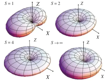
Calculations of ␤V共␽,␸兲= const− lnWS共␽,␸兲 关V共␽,␸兲

has the meaning of an “effective” free energy potential兴 are shown in Fig.1 for various values ofSand␴

⬘

=␴S2= 5 and h=␰/共2␴S兲= 0.1. In the classical limit 共S→⬁, ␰S= const =␰

⬘

, ␴S2_{= const=␴}

_⬘

_{兲, the effective potential V共␽,␸兲} be-comes the classical free energyVcl共␽,␸兲given by

␤Vcl共␽,␸兲= const −␴

⬘共cos

2␽+ 2hcos␸sin␽兲,

which is also shown in Fig.1for comparison. The effective potentialV共␽,␸兲 共just as the classical free energyVcl共␽,␸兲兴

has two equivalent minima and one saddle point in the plane

␸= 0 at ␽=␲/2; the potential characteristics 共such as the shape and barrier heights兲 strongly depend on S, e.g., the smallest barrier height increases with increasingSfrom 0共at S=1₂兲to its classical value␴

⬘

共1 −h2_兲.

S= 1

X

Z S= 2 Z

X S→ ∞

S= 4 Z

X Z

[image:6.612.347.519.58.191.2]

X

V. BIAXIAL SYSTEM

We now calculate the Wigner function of a biaxial spin system with Hamiltonian

␤HˆS= −␴SˆZ2+␦共SˆX2−SˆY2兲 共29兲

commonly used to describe the magnetic properties of an octanuclear iron共III兲 molecular cluster Fe8.5,42 _{For Fe8, S} = 10, ␴T= 0.275 K, and ␦T= 0.046 K.42 _{The density matrix}

␳ˆS=e−␤H ˆ

S/_Z

Scan be given in simple closed form for smallS.

For example, forS=1₂,S= 1, etc., we have after matrix alge-bra

␳ˆ_1/2= e ␴/4

Z1/2

Iˆ, 共30兲

␳ˆ₁= 1 Z1

关Iˆ+共e␴cosh␦− 1兲SˆZ

2

−e␴sinh␦共SˆX

2 −SˆY

2_兲兴 ,

共31兲

␳ˆ_3/2= e

5␴/4_sinh

冑

_3␦2_+␴2

Z3/2

冑

3␦2+␴2 兵␴SˆZ

2 −␦共SˆX

2 −SˆY

2_兲

+关

冑

3␦2+␴2coth

冑

3␦2+␴2− 5␴/4兴Iˆ其, 共32兲 where Z1/2= 2e␴/4, Z1= 1 + 2e␴cosh␦, and Z3/2 = 4e5␴/4_cosh

冑

₃␦2_+␴2_{. The corresponding equations for} WS共␽,␸兲are

W1/2共␽,␸兲= 1/2, 共33兲

W₁共␽,␸兲= 1 2Z1

关sin2␽+e␴cosh␦共1 + cos2␽兲

−e␴sinh␦sin2␽cos 2␸兴, 共34兲

W_3/2共␽,␸兲= 1 4+

3 tanh

冑

3␦2+␴2 8

冑

3␦2+␴2 关␴cos

2_␽−␦sin2_{␽cos 2␸}

−␴/3兴. 共35兲

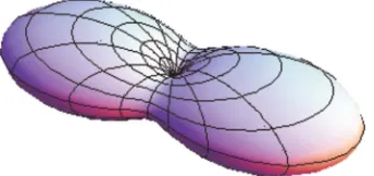
The effective potential ␤V共␽,␸兲= const− lnWS共␽,␸兲 is

shown in Fig.2forS= 2,␴

⬘

=␴S2= 5, and␦

⬘

=␦S2= 5. In the classical limit共S→⬁, ␦

⬘

=␦S2_{= const, and ␴S}2_{= const=␴}

_⬘

_兲, the effective potential V共␽,␸兲 again tends to the classical free energyVcl共␽,␸兲 given by

␤Vcl共␽,␸兲= const −共␴

⬘

cos2␽−␦

⬘

cos 2␸sin2␽兲.

The effective potential V共␽,␸兲 关just as Vcl共␽,␸兲兴 has two

equivalent minima and two saddle points in the planeXZat

␽=␲/2; potential characteristics共such as the shape and bar-rier heights兲 again strongly depend on S. In particular, the barrier height increases with increasingSfrom 0共atS= 1/2兲 to its classical value␴

⬘

.

VI. CUBIC SYSTEM

Finally, we calculate the Wigner function of a cubic spin system in a longitudinal dc field with Hamiltonian

␤HˆS= −␰SZ−␴共SˆX4+SˆY4+SˆZ4兲/2,

where ␴ is the dimensionless anisotropy parameter, which may be either positive or negative. For smallS, the density matrix␳ˆS=e−␤H

ˆ S/_Z

Scan again be given in closed form. For

example, forS= 1/2,S= 1, etc., we have

␳ˆ_1/2=e 3␴/32

Z1/2

关Iˆcosh共␰/2兲+ 2SˆZsinh共␰/2兲兴, 共36兲

␳ˆ₁= e ␴

Z1

关Iˆ+ sinh␰SˆZ+ 2 sinh2共␰/2兲SˆZ

2_{兴, 共37兲}

␳ˆ_3/2=e 123␴/32

Z3/2

再

1

8关9 cosh共␰/2兲− cosh共3␰/2兲兴Iˆ

+ 1

12关27 sinh共␰/2兲− sinh共3␰/2兲兴SˆZ+ 2 cosh共␰/2兲

⫻关sinh共␰/2兲SˆZ兴2+

4

3关sinh共␰/2兲SˆZ兴

3

冎

_{, 共38兲}

␳ˆ₂= 1 Z2

再

冉

e12␴−6␴

␰ R

冊

Iˆ+

1 6共8e

9␴_{sinh␰−R兲Sˆ}

Z

+ 1 12

冉

16e

9␴_{cosh␰− 15e}12␴_−P+93␴ 4␰ R

冊

SˆZ

2

−1 6共2e

9␴_{sinh␰−R兲Sˆ}

Z

3

+ 1 12

冉

3e

12␴_{− 4e}9␴_cosh␰+P−9␴ 4␰R

冊

⫻SˆZ

4 + ␴

4␰R共SˆX 4

+SˆY

4_兲

冎

, 共39兲

where

Z1/2= 2 cosh共␰/2兲e3␴/32, Z1=共1 + 2 cosh␰兲e␴,

Z3/2= 4 cosh共␰/2兲cosh␰e123␴/32,

Z2=e9␴共e3␴+ 2 cosh␰+ 2e3␴/2cosh关2␰

冑

1 +共3␴/4␰兲2兴兲,

[image:7.612.90.262.62.143.2]

P=e21␴/2cosh关2␰

冑

1 +共3␴/4␰兲2兴, FIG. 2.共Color online兲3D plot of␤V共␽,␸兲forS= 2,␴⬘= 5, and

R=e21␴/2sinh关2␰

冑

1 +共3␴/4␰兲2兴/

冑

1 +共3␴/4␰兲2. The corresponding equations forWS共␽,␸兲are

W1/2共␽,␸兲=e3␴/32关cosh共␰/2兲+ sinh共␰/2兲cos␽兴/Z1/2, 共40兲

W₁共␽,␸兲=e␴关cosh共␰/2兲+ sinh共␰/2兲cos␽兴2/Z₁, 共41兲

W3/2共␽,␸兲=e123␴/32关cosh共␰/2兲+ sinh共␰/2兲cos␽兴3/Z3/2, 共42兲

W2共␽,␸兲= 1 8Z2

兵2e9␴sin2␽关4 sin␰cos␽

+ cosh␰共3 + cos 2␽兲兴+ 3e12␴sin4␽ +P共8 cos2␽+ sin4␽兲

+ 4R关cos␽+ cos3_{␽+共3␴/16␰兲cos 4␸sin}4_␽兴其. 共43兲 For␰= 0, Eq.共43兲yields

W2共␽,␸兲= 1

2共3 + 2e3␴兲关1 +e

3␴_+共e3␴_{− 1兲共sin}2_2␽

+ sin4␽sin22␸兲/4兴. 共44兲 The effective potential ␤V共␽,␸兲= const− lnWS共␽,␸兲 is

shown in Fig. 3 for ␴

⬘

=␴S4=⫾8, ␰= 0, and S= 4. In the classical limit共S→⬁, ␴S4_{= const=␴}

_⬘

_{兲, the effective} poten-tial once more tends to the classical free energy Vcl共␽,␸兲

given by

␤Vcl共␽,␸兲= const +␴

⬘

共sin22␽+ sin4␽sin22␸兲.

For positive anisotropy constant ␴⬎0, the cubic potential has 6 minima共wells兲, 8 maxima, and 12 saddle points. For

␴⬍0, the maxima and minima are interchanged. The poten-tial characteristics 共such as the shape and barrier heights兲 again strongly depend onS. In particular, the smallest barrier height again increases with increasingS from 0共atS=1₂兲to its classical value␴

⬘

.

It is apparent from the examples chosen that the Wigner– Stratonovich transformation allows one to calculate the equi-librium phase-space distribution共Wigner function兲via its fi-nite Fourier series representation for any given anisotropy. The results may be used to estimate the reversal time of the magnetization from TST as well as to include thermal effects

in the quantum generalization of Thiaville’s calculation of switching field curves and/or surfaces. However, in accor-dance with the stated objectives of the paper we shall first demonstrate how the phase-space representation of the Hamiltonian operator for a given spin system may be used to calculate switching field curves as a function of spin at zero temperature.

VII. SWITCHING FIELD CURVES

We recall that the first calculation of the magnetization reversal of single-domain ferromagnetic particles with uniaxial anisotropy subjected to an applied field was made by Stoner and Wohlfarth7 _{with the hypothesis of coherent} rotation of the magnetization and zero temperature so that thermally induced switching between the potential minima is ignored. In the simplest uniaxial anisotropy as considered by them, the magnetization reversal occurs at the particular value of the applied field共switching field兲which destroys the bistable nature of the potential. The parametric plot of the parallel vs the perpendicular component of the switching field then yields the famous astroids. In the general approach to the calculation of switching curves via the geometrical method of Thiaville,8 _{the switching field curves or surfaces} may be constructed for particles with arbitrary anisotropy at zero temperature. These calculations again, however, pertain to particles where the magnetization may be represented by a single macrospin共coherent rotation of the magnetization兲. In order to generalize Thiaville’s geometrical method8 _to in-clude spin size effects, we have to calculate the Weyl symbol 共c number兲 HS共␽,␸兲 corresponding to the Hamiltonian HˆS,

which is defined as

HS共␽,␸兲= Tr关HˆSwˆ−1共␽,␸兲兴

=

冑

4␲ 2S+ 1Tr

冋

H

ˆ

S

兺

L=0 2S

兺

M=−L L

CS,S,L,0

S,S

Y_L*_,MTˆL共,M S兲

册

.

共45兲 Then treating the c-number representation HS共␽,␸兲 as an

arbitrary potential energy one may in principle calculate the switching fields using Thiaville’s method.8_{We illustrate this} by considering the uniaxial

␤HˆS un

= −␴1SˆZ

2

, 共46兲

biaxial

␤HˆS bi

= −␴1SZ

2 +␦共SˆX

2 −SˆY

2_{兲, 共47兲}

cubic

␤HˆS cub

= −␴2共SˆX

4 +SˆY

4 +SˆZ

4_兲/

2, 共48兲

and mixed anisotropy

␤HˆS mix

= −␴1SˆZ

2 −␴2SˆZ

4

[image:8.612.91.256.63.144.2]

+␹共Sˆ₊4+Sˆ₋4兲 共49兲 Hamiltonians. The mixed anisotropy Hamiltonian 共49兲 is commonly used to describe the magnetic properties of the dodecanuclear manganese molecular cluster Mn12.42 _For FIG. 3. 共Color online兲 3D plot of␤V共␽,␸兲 for positive 共left兲

Mn12, S= 10, ␴1T= 0.56 K, ␴2T= 1.1⫻10−3 K, and ␹T =⫾3⫻10−5 _K.42

The Weyl symbolsHS un_共␽

,␸兲,HS bi_共␽

,␸兲,HS cub_共␽

,␸兲, and HS

mix_共␽

,␸兲 corresponding to the Hamiltonian operators 共46兲–共49兲 can be calculated from the general finite Fourier series representation equation共45兲noting Eqs.共16兲and共19兲. We obtain after some algebra

HS un

= −␴1S共S− 1/2兲cos2␽−␴1S/2, 共50兲

HS bi

= −␴1S关共S− 1/2兲共cos2␽−⌬cos 2␸sin2␽兲+ 1/2兴, 共51兲

HS cub

= −␴2S共2S3+ 3S− 1兲/4 +␴2S共S− 1兲共S− 1/2兲共S− 3/2兲

⫻共sin2_{2␽+ sin}4_␽sin2_{2␸兲/4, 共52兲} and

HS mix

= −S

4关2␴1+␴2共3S− 1兲兴−S共S− 1/2兲关␴1+␴2共3S− 2兲兴

⫻cos2␽−1

2S共S− 1兲共S− 3/2兲共S− 1/2兲关2␴2cos 4_␽

−␹sin4␽cos 4␸兴, 共53兲

respectively, where ⌬=␦/␴₁. If we further suppose that a uniform external magnetic field H is applied along thex-z plane, the Zeeman term operator ␤HˆS= −␰sin␺SˆX

−␰cos␺SˆZtransforms to the phase space as

␤HS= −␰Scos共␽−␺兲, 共54兲

where␺ is the angle between the applied fieldHand theZ axis. Thus the switching fieldshun,hbi, and hcub in thex-z

plane 共i.e., for ␸= 0兲can be calculated from Eqs.共50兲–共52兲 so that

hun=Qunhun cl

, hbi=Qbihbi cl

, andhcub=Qcubhcub cl

, 共55兲 where the quantum correction factorsQun,Qbi, andQcuband

corresponding classical switching fieldshun cl

,hbi cl

, andhcub cl

are

Qun=Qbi=共S− 1/2兲/S, 共56兲

Qcub=共S− 1/2兲共S− 1兲共S− 3/2兲/S3,

hun cl

=共sin3␺,cos3␺兲,

hcub cl

=关sin3␺共3 cos 2␺+ 2兲,cos3␺共3 cos 2␺− 2兲兴,

hbi cl

=共sin␺关2⌬+f共␺兲兴,cos␺关2 −f共␺兲兴兲, 共57兲 and f共␺兲=共1 +⌬兲sin2_{␺+兩2⌬−共1 +⌬兲sin}2_{␺兩. For mixed} an-isotropy, the corresponding equation for the switching field

hmix is much more complicated and must be calculated

nu-merically. The parametric plots of the parallelhZvs the

per-pendicularhX component of the switching field yield the

as-troids and hypocycloids for uniaxial and cubic systems, respectively, along with the corresponding quantum

correc-tion factors关see Figs.4共a兲and4共c兲兴. For biaxial and mixed anisotropies, the behavior of the switching fields is much more involved and is shown in Figs.4共b兲and4共d兲. In general the figures indicate that the switching field amplitudes in-creasemarkedly with increasing S tending to their classical limiting values asS→⬁ corresponding to diminishing tun-neling effects as that mechanism is gradually shut off.

We emphasize that the above calculations because they are entirely based on the phase-space representation of the Hamiltonian operator ignore thermal effects. To account for these it is necessary to estimate the temperature dependence of the reversal time of the magnetization which may be ac-complished using transition state theory共TST兲. The estima-tion of the reversal time of magnetizaestima-tion in the context of TST is, probably, the most promising application of the phase-space approach. TST as we shall now see again in-volves only the quantum equilibrium distributions, which we have calculated in the preceding sections.

VIII. TRANSITION STATE THEORY REVERSAL TIME OF THE MAGNETIZATION

We have mentioned that TST affords the simplest possible description of quantum corrections to thermally activated de-cay due to thermal agitation. In applying TST to classical spins 共i.e., magnetic moments ␮兲, in order to evaluate the escape rate from a metastable orientationi to another meta-stable orientationj, we suppose that the free energyV共␽,␸兲 of a magnetic moment ␮ has a multistable structure with minima at ni andnj separated by a potential barrier with a

saddle point atn₀. In the low temperature limit共high barrier

-1 1

-1 1

-1 1

-1 1

-1 1

-1 1

-1 1

-1 1

(a) (b)

(c) _(d)

hZ

hZ

hX

hX

hZ

hZ

hX

[image:9.612.320.558.61.300.2]

hX

FIG. 4. Spin dependence of switching field curves for 共a兲 uniaxial, 共b兲 biaxial at ␴₁/␦= 0.25, 共c兲 cubic, and 共d兲 mixed 共at ␴1/␴2= 0.5 and␹= 0兲anisotropies calculated atS= 2共solid lines兲, 5

approximation兲, as far as TST is concerned, the escape rate

⌫clmay be estimated as

⌫cl⬃I0

cl_/

Zi cl

, 共58兲

where Zi cl_⬃兰

welle−␤V共␽,␸兲sin␽d␽d␸ is the well partition

function and I₀cl is the total current of the 共magnetization兲 representative points at the saddle point. In order to evaluate the well partition functionZi

cl

, we suppose10,11 _{that the free} energyVnear the minimum nican be approximated as

Vcl=Vcl共nk兲+

1 2关c1共

k_兲共

u₁共k兲兲2+c₂共k兲共u₂共k兲兲2兴, 共59兲

where共u₁共i兲,u₂共i兲, u₃共i兲兲denote the direction cosines of␮ near

ni,c₁共 i兲

=⳵2_V

cl/⳵u₁共 i兲2

, andc₂共i兲=⳵2_V

cl/⳵u₂共 i兲2

. Hence

Zi cl_⬃

冕

well

e−␤Vcl共u1共 i兲

,u₂共i兲兲

du₁共i兲du₂共i兲⬃ 2␲

␤

冑

c₁共i兲c₂共i兲e −␤V共n_i兲

.

共60兲

The total currentI₀clmay be estimated as共by supposing that thexaxis of the local coordinate system at the saddle point

n0is in the same direction as the probability currentJ0over the saddle and recalling that the Boltzmann distribution holds everywhere兲

I₀cl⬃

冕

saddle

␪共u₁共0兲兲␦共u₂共0兲兲J0共u1共 0兲_,u

2

共0兲_兲e−␤V_cl共u₁共0兲,u₂共0兲兲

du₁共0兲du₂共0兲

⬇ ␥

␮␤

冕

saddle

de−␤Vcl⬇ ␥

␮␤e−␤Vcl共n0兲, 共61兲

where J₀= −共␥/␮兲⳵Vcl/⳵u1共

0兲_{=共␥/␤␮兲⳵ln共e}−␤V_cl兲/⳵u

1 共0兲 _{is a} divergence-free current density at the saddle point and␪ is the unit step function. Hence, noting Eqs.共60兲and共61兲, Eq. 共58兲yields the classical TST formula for spins

⌫cl⬃ 共␻i/2␲兲e−␤⌬V cl

, 共62兲

where the attempt frequency

␻i=␥冑c1共

i_兲

c₂共i兲/␮ 共63兲

is the well 共precession兲 frequency and ⌬Vcl=Vcl共n0兲 −Vcl共ni兲is the potential barrier height共the determination of

which involves detailed knowledge of the energy landscape兲. The quantum escape rate⌫i for a spin from a metastable

orientation i to another metastable orientation j as deter-mined by quantum TST may be given by an equation similar to Eq.共58兲, viz.,

⌫i⬃I0/Zi. 共64兲

However, the well partition functionZiand the total current

over the saddle point I0 must now be evaluated using the equilibrium phase-space distribution function W共␽,␸兲 in-stead of the Boltzmann distribution⬃exp关−␤Vcl共␽,␸兲兴. Just

as uniaxial systems,36 _{the distribution W can be} approxi-mated in the vicinity of the metastable minimumni by the

spin in a uniform field or Zeeman energy distribution given by Eq.共20兲, viz.,

WS共␽,␸兲=WS共ni兲e−S␰i关cosh共␰i/2兲+ sinh共␰i/2兲Fi共␽,␸兲兴2S,

共65兲 where Fi共␽,␸兲=␥X_isin␽cos␸+␥Y_isin␽sin␸+␥Z_icos␽

withFi共␽i,␸i兲= 1,␥X_i,␥Y_i,␥Z_iare the direction cosines of the

effective field Hi= −⳵V/⳵␮ in the vicinity of minimum ni,

and␮=ប␥S is the magnetic moment,␰i=␤ប兩␻i兩is the

nor-malized precession frequency␻i=␥Hi. All the foregoing

re-sults rely on the fact that the dynamics of a spin nearni at

low temperatures comprise steady precession in theeffective magnetic field Hi in the well. The precession frequency ␻i

can be estimated from the well angular frequency 共i.e., at-tempt frequency兲Eq.共63兲, where the coefficientsc₁共i兲andc₂共i兲 are determined from the Taylor series expansion of the Weyl symbolHS共␽,␸兲of the HamiltonianHˆSof a spin

HS=HS共nk兲+

1 2关c1共

k兲_共

u1共

k兲_兲2_+c 2 共k兲_共

u2共

k兲_兲2_{兴 共66兲}

共␻ican also be found experimentally by measuring the

criti-cal switching field surface and then applying Thiaville’s geo-metrical methods兲. Noting Eq.共21兲, we can now estimate the well partition function as

Zi⬃WS共ni兲e−S␰i

冕

well

关cosh共␰i/2兲

+ sinh共␰i/2兲Fi共␽,␸兲兴2Ssin␽d␽d␸

= 4␲WS共ni兲e−S␰i

sinh关共S+ 1/2兲␰i兴

共2S+ 1兲sinh共␰i/2兲

⬇ 2␲WS共ni兲

共S+ 1/2兲共1 −e−␰i兲.

共67兲 The currentI0 at the saddle pointn0 may also be estimated just as in Eq.共61兲, viz.,

I0⬃

冕

top

␪共u₁共0兲兲␦共u₂共0兲兲J0共u1共 0兲

,u₂共0兲兲W共u₁共0兲,u₂共0兲兲du₁共0兲du₂共0兲

⬃␥W共n0兲/共␮␤兲, 共68兲

where J0= −共␥/␮兲⳵V/⳵u1 共0兲

=共␥/␤␮兲⳵lnW/⳵u₁共0兲. Hence we have the TST escape rate for spins as determined from Eqs. 共64兲,共67兲, and 共68兲, viz.,

⌫i⬃

␥共S+ 1/2兲共1 −e−␰i兲

2␲␮␤

WS共n0兲 WS共ni兲

. 共69兲

To compare this equation with the classical TST equation 共62兲, we can write the resulting escape rate formula for spins in the canonical form

⌫⬃ 共␻i/2␲兲⌶e−␤⌬V, 共70兲

where

⌶=共S+ 1/2兲共1 −e−␰i兲/_S␰

i and ␤⌬V= ln关WS共n0兲/WS共ni兲兴

are, respectively, thequantum correctionfactor andeffective barrier height, i.e., the argument of the exponential. Here both ␤⌬V and ⌶ strongly depend on the spin number S yielding␤⌬V→␤⌬Vcland⌶→1, respectively, in the

␻i=␴共2S− 1兲/共ប␤兲,

⌶= 2S+ 1

2␴S共2S− 1兲关1 −e

−␴共2S−1兲_兴,

␤⌬V=␴S2− ln共2S兲! 22S m

兺

=−S

S

e␴m2 共S+m兲!共S−m兲!.

Just as the classical case, having evaluated the escape rate⌫i

for a particular anisotropy, one can calculate the reversal time at finite temperatures. In particular, by equating reversal time to measuring time this calculation allows one to esti-mate the switching field curves at finite temperatures just as the classical theory.43 _{One should remember, however, that} TST always implies that the dissipation to the bath does not affect the escape rate. Nevertheless, the results should still apply in awide range of dissipationfor which thermal noise is sufficiently strong to thermalize the escaping system yet insufficient to disturb the thermal equilibrium in the well, i.e., an equilibrium distribution still prevails everywhere in-cluding the saddle point. In the context of the classical Kramers escape rate theory,16_{this is the so called}

intermedi-ate dampingcase.

IX. DISCUSSION

We have amply demonstrated that the phase-space method formally representing the quantum mechanics of spins as a statistical theory in the classical configuration space of polar angles 共␽,␸兲 共which are now the canonical variables兲 may be used to construct equilibrium distribution共Wigner兲 func-tions for nonaxially symmetric model spin Hamiltonians. The Wigner function may be represented using the Wigner– Stratonovich map as a Fourier series just as the correspond-ing classical orientational distribution and transparently re-duces to it in the classical limit. Moreover, relevant quantum mechanical averages may be calculated in a manner analo-gous to the corresponding classical averages using the Weyl symbol of the appropriate quantum operator. The Wigner functions can now be applied to important magnetic prob-lems such as the equilibrium magnetization, switching, and hysteresis curves, which require only a knowledge of equi-librium distributions. Two examples given in the paper are the estimation of the reversal time of the magnetization using TST and the spin dependence of the switching fields as gen-eralized to arbitrary magnetocrystalline anisotropy-Zeeman energy Hamiltonians by Thiaville.8 _{In the latter case, it is} obvious that the behavior of the switching field curves and/or surfaces as a function of spin size may be determined using the Weyl symbol of the relevant Hamiltonian and the phase-space representation generated by the Wigner–Stratonovich map just as the solution of the classical problem. This fact is important particularly from an experimental point of view as the transition between magnetic molecular cluster and single-domain ferromagnetic nanoparticle behavior is essentially demarcated via the hysteresis loops and the corresponding switching fields.5_{Yet another advantage of the phase-space} representation is that via TST as corrected for spin size

ef-fects共which is readily apparent from that representation兲it is possible to predict the temperature dependence of the switch-ing fields and correspondswitch-ing hysteresis loops within the limi-tations imposed by TST. This is likely to be of interest in experiments seeking evidence for macroscopic quantum tun-neling where the temperature dependence of the loops is cru-cial as the loops are used5 _{to demarcate tunneling behavior} from thermal agitation behavior.