Graph Convolutional Networks for Named Entity Recognition

Proceedings of the 16th International Workshop on Treebanks and Linguistic Theories (TLT16), pages 37–45, Prague, Czech Republic, January 23–24, 2018. Distributed under a CC-BY 4.0 licence. 2017.

Graph Convolutional Networks for Named Entity Recognition

Cetoli, Alberto Bragaglia, Stefano O’Harney, Andrew Daniel Sloan, Marc

Context Scout

{alberto, stefano, andy, marc}@contextscout.com

Abstract

In this paper we investigate the role of the dependency tree in a named entity recognizer upon using

a set of Graph Convolutional Networks (GCNs). We perform a comparison among different Named

Entity Recognition (NER) architectures and show that the grammar of a sentence positively influ-ences the results. Experiments on theOntoNotes 5.0dataset demonstrate consistent performance improvements, without requiring heavy feature engineering nor additional language-specific knowledge.1

1 Introduction and Motivations

The recent article byMarcheggiani and Titov(Marcheggiani and Titov,2017) opened the way for a novel method in Natural Language Processing (NLP). In their work, they adopt aGCN(Kipf and Welling,2016) approach to perform semantic role labeling, improving upon previous architectures. While their article is specific to recognizing the predicate-argument structure of a sentence, their method can be applied to other areas ofNLP. One example isNER.

High performing statistical approaches have been used in the past for entity recognition, notably

Markovmodels (McCallum et al.,2000), Conditional Random Fields (CRFs) (Lafferty et al.,2001), and Support Vector Machines (SVMs) (Takeuchi and Collier,2002). More recently, the use of neural networks

has become common inNER.

The method proposed by Collobert et al. (Collobert et al., 2011) suggests that a simple

feed--forward network can produce competitive results with respect to other approaches. Shortly thereafter,

Chiu and Nichols (Chiu and Nichols, 2015) employed Recurrent Neural Networks (RNNs) to address

the problem of entity recognition, thus achieving state-of-the-art results. Their key improvements were twofold: using a bi-directional Long Short-Term Memory (LSTM) in place of a feed-forward network and concatenating morphological information to the input vectors.

Subsequently, various improvements appeared: using a CRF as a last layer (Huang et al., 2015) in

place of asoftmaxfunction, a gated approach to concatenating morphology (Cao and Rei,2016) and

predicting nearby words (Rei,2017). All such methods, however, understand text as a one dimensional collection of input vectors; any syntactic information – namely the parse tree of the sentence – is ignored.

We believe that dependency trees and other linguistic features play a key role on the accuracy ofNER

and thatGCNscan grant the flexibility and convenience of use that we desire. In this paper our contribution is twofold: on one hand, we introduce a methodology for tackling entity recognition withGCNs; on the other hand we measure the impact of using dependency trees for entity classification upon comparing the results with prior solutions. At this stage our goal is not to beat the state-of-the-art but rather to quantify the effect of our novel architecture.

1_{A version of this system can be found athttps://github.com/contextscout/gcn_ner.}

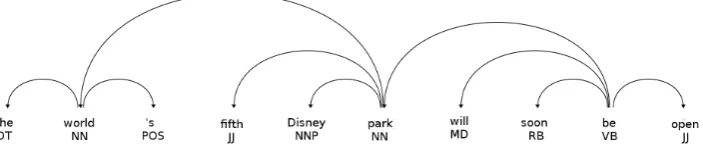
Figure 1: An example sentence along with its dependency graph. GCNspropagate the information of a node to its nearest neighbours.

As a final note, we notice that treebanks offer more information than a one dimensional sequence of words. This information is not used in conventionalRNNssystems. Our paper opens the way for exploiting the syntax and dependency structures available in a treebank.

The remainder of the article is organized as follows: in Section2we introduce the theoretical framework for our methodology, then the features considered in our model and eventually the training details. Section 3describes the experiments and presents the results. We discuss relevant works in Section4and draw the conclusions in Section5.

2 Methods and Materials

2.1 Theoretical Aspects

Graph Convolutional Networks (Kipf and Welling,2016) operate on graphs by convolving the features of

neighbouring nodes. AGCNlayer propagates the information of a node onto its nearest neighbours. By

stacking togetherNlayers, the network can propagate the features of nodes that are at mostNhops away. While the original formulation did not include directed graphs, they were further extended in

Marcheggiani and Titovto be used on directed syntactic/dependency trees. In the following we rely on

their work to assemble our network.

EachGCNlayer creates new node embeddings by using neighbouring nodes and these layers can be

stacked upon each other. In the undirected graph case, the information at thekstlayer is propagated to the next one according to the equation

hk_v+1= ReLU



 X

u∈N(v)

Wkhk_u+bk



, (1)

whereuandvare nodes in the graph. N is the set of nearest neighbours of nodev, plus the nodevitself. The vectorhk_urepresents nodeu’s embeddings at thekstlayer, whileW andbare a weight matrix and a bias – learned during training – that map the embeddings of nodeuonto the adjacent nodes in the graph;

hubelongs toRm,W∈Rm×mandb∈Rm.

Following the example in Marcheggiani and Titov, we prefer to exploit the directness of the graph

in our system. Our inspiration comes from the bi-directional architecture of stackedRNNs, where two different neural networks operate forward and backward respectively. Eventually the output of theRNNs

is concatenated and passed to further layers.

In our architecture we employ two stackedGCNs: One that only considers the incoming edges for each node

←−

hk_v+1= ReLU



 

X

u∈←N−(v) ←−

Wkhk_u+←−bk 



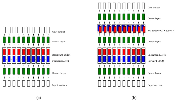
Input vectors Dense Layer Forward LSTM Backward LSTM Dense layer CRF output

(a)

Input vectors Dense Layer Forward LSTM Backward LSTM Dense layer Fw and bw GCN layer(s) Dense layer CRF output

(b)

Figure 2: bi-directional architectures:(a)LSTM; and,(b)GCNlayers.

and one that considers only the outgoing edges from each node

− →

hk_v+1= ReLU



 

X

u∈−→N(v) −→

Wkhk_u+−→bk 



. (3)

AfterN layers the final output of the twoGCNsis the concatenation of the two separated layers

hN_v =−→h_vN⊕←−hN_v . (4)

In the following, we refer to the architecture expressed by Equation4as abi-directionalGCN_.

2.2 Implementations Details

2.2.1 Using the dataset

We employ theOntoNotes 5.0dataset (Weischedel,2013) for training and testing. This dataset annotates various genres of text for the purpose of entity recognition and co-reference resolution. The annotated sentences are provided with Part-of-Speech (PoS) tags and syntactic information. While we include the

PoStags in our tests, the Phrase Structure Grammar (PSG) structures in theOntoNotes 5.0are not used. The dependency graphs that are fed to the graph convolutional network are instead computed by an external parser,Spacy v1.8.2(Honnibal and Johnson,2015).

In principle we could have translated the syntactic trees in the dataset to dependency graphs using - for

example - the CCGBank manual (Hockenmaier and Steedman,2007). We will investigate this approach

in future works, while this paper lays down the technique for boosting entity recognition usingGCNs.

2.2.2 Models

Our architecture is inspired by the work of Chiu and Nichols (Chiu and Nichols, 2015),

Huang et al. (Huang et al., 2015), and Marcheggiani and Titov (Marcheggiani and Titov, 2017). We

aim to combine a Bi-directional Long Short-Term Memory (Bi-LSTM) model withGCNs, usingCRFas the last layer in place of asoftmaxfunction.

We employ seven different configurations by selecting from two sets ofPoStags and two sets of word

embedding vectors. All the models share a bi-directionalLSTMwhich acts as the foundation upon which

Bi-LSTM We use a bi-directionalLSTMstructured as in Figure2(a). The output is mediated by two fully connected layers ending in aCRF(Huang et al.,2015), modelled as a Viterbi sequence. The best results

in thedev setofOntoNotes 5.0were obtained upon staking twoLSTMlayers, both for the forward and

backward configuration. This is the number of layers we keep in the rest of our work. This configuration – when used alone – is a consistency test with respect to the previous works. As seen in Table1, our findings are compatible with the results in (Chiu and Nichols,2015).

Bi-GCN In this model, we use the architecture created in (Marcheggiani and Titov,2017) where aGCN

is applied on top of aBi-LSTM. This system is shown in Figure2(b)(right side). The best results in thedev

setwere obtained upon using only oneGCNlayer, and we use this configuration through our models. We

employ two different embedding vectors for this configuration: one in which only word embeddings are fed as an input, the other one wherePoStag embeddings are concatenated to the word vectors.

Input vectors We use three sets of input vectors. First, we simply employ the word embeddings found in theGlovevectors (Pennington et al.,2014):

x_input=x_glove. (5)

In the following, we employ the300dimensional vector from two different distributions: one with1M

words and another one with2.2M words. Whenever a word is not present in theGlovevocabulary we use the vector corresponding to the word “entity” instead.

The second type of vector embeddings concatenates theGloveword vectors withPoStags embeddings.

We use randomly initialized Part-of-Speech embeddings that are allowed to fine-tune during training:

xinput=xglove⊕xPoS. (6)

The final quality of our results correlates to the quality of our Part-of-Speech tagging. In one batch we use the manually curatedPoStags included in theOntoNotes 5.0dataset (Weischedel,2013) (PoS(gold)). These tags have the highest quality.

In another batch, we use thePoStagging inferred from the parser (PoS(inferred)) instead of using the manually tagged ones. ThesePoStags are of lower quality. An external tagger might provide a different number of tokens compared to the ones present in the training and evaluation datasets. This presents a challenge. We skip these sentences during training (1602 sentences out of 112300), while considering the entities in such sentences as incorrectly tagged during evaluation.

Finally, we add the morphological information to the feature vector for the third type of word embed-dings. The reason – explained in (Cao and Rei,2016) – is that out-of-vocabulary words are handled badly whilst using only word embeddings:

xinput=xglove⊕xPoS⊕xmorphology. (7)

We employ a bi-directionalRNNto encode character information. The end nodes of theRNNare concate-nated and passed to a dense layer, which is integrated to the feature vector along with the embeddings and

PoSinformation. In order to speed up the computation, we truncate the words by keeping only the first 12 characters. This operation is only done when computing the morphology vector, the word embeddings still refer to the full word. Truncation is not commonly done, as it hinders the network’s performance; we leave further analysis to following works.

Dropout In order to tackle over-fitting, we apply dropout to all the layers on top of the LSTM. The probability to drop a node is set at20%for all the configurations. The layers that are used as input to the

LSTMdo not use dropout.

Network output At inference time, the output of the network is a19-dimensional vector for each input

word. This dimensionality comes from the18tags used inOntoNotes 5.0, with an additional dimension

which expresses the absence of a named entity. No Begin, Inside, Outside, End, Single (BIOES) markings

are applied; at evaluation time we simply consider a name chunk as a contiguous sequence of words

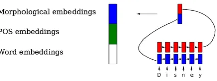
Figure 3: Feature vector components. Our input vectors have up to three components: the word

embeddings, thePoSembeddings, and a morphological embedding obtained through feeding each word

to aBi-LSTMand then concatenating the first and last hidden state.

2.2.3 Training

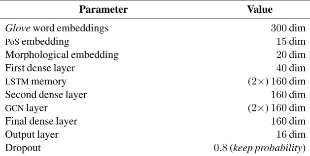
We useTensorFlow(Abadi et al.,2015) to implement our neural network. Training and inference is done at the sentence level. The weights are initialized randomly from the uniform distribution and the initial state of theLSTMsare set to zero. The system uses the configuration in AppendixA.

The training function is theCRFloss function as explained in (Huang et al., 2015). Following their notation, we define[f]i,t as the matrix that represents the score of the network for thetth word to have

theithtag. We also introduceAij as the transition matrix which stores the probability of going from tag

ito tagj. The transition matrix is usually trained along with the other network weights. In our work we preferred instead to set it as constant and equal to the transition frequencies as found in the training dataset.

The functionf is an argument of the network’s parametersθand the input sentence[x]T

1 (the list of

embeddings with lengthT). Let the list ofT training labels be written as[i]T

1, then our loss function is

written as

S [x]T

1,[i]T1,θ,Aij

−X

[j]T 1

exp [x]T

1,[j]T1,θ,Aij+[f][i]t,t

, (8)

where

S _[x]T₁,[i]T₁,θ,Aij

=

T

X

1 A_[i]t

−1,[i]t+f(θ,Aij)

. (9)

At inference time, we rely on the Viterbi algorithm to find the sequence of tokens that maxi-mizes S [x]T

1,[i]T1,θ,Aij

. We apply mini-batch stochastic gradient descent with the Adam

opti-miser (Kingma and Ba,2014), using a learning rate fixed to10−4.

3 Experimental Results

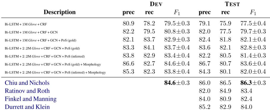
In this section, we compare the different methods applied and discuss the results. The scores in Table12 are presented as an average of6runs with the error being the standard deviation; we keep only the first significant digit of the errors, approximating to the nearest number.

The results show an improvement of2.2±₀.5%upon using aGCN, compared to the baseline result of a bi-directionalLSTM alone (1st _{row). When concatenating the goldPoStag embedding in the input}

vectors, this improvement raises to4.6±0.6%. However, the gold tags in theOntoNotes 5.0only refer to the sentences within the dataset. Therefore, the performance of the system on new sentences must rely on inferredPoStags.

The F1 score improvement for the system while using inferred tags (from the parser) is lower:

3.2±0.6%.

DEV TEST

Description prec rec F1 prec rec F1

Bi-LSTM +1MGlove+ CRF 80.9 78.2 79.5±0.3 79.1 75.9 77.5±0.4 Bi-LSTM +1MGlove+ CRF + GCN 82.2 79.5 80.8±0.3 82.0 77.5 79.7±0.3

Bi-LSTM +1MGlove+ CRF + GCN + PoS (gold) 82.1 83.7 82.9±0.3 82.4 81.8 82.1±0.4 Bi-LSTM +2._2MGlove+ CRF + GCN + PoS (gold) 83.3 84.1 83.7±0.4 83.6 82.1 82.8±0.3 Bi-LSTM +2.₂MGlove+ CRF + GCN + PoS (inferred) 83.8 82.9 83.4±0.4 82.2 80.5 81.4±0.3

Bi-LSTM +2._2MGlove+ CRF + GCN + PoS (gold) + Morphology 86.6 82.7 84.6±0.4 86.7 80.7 83.6±0.4 Bi-LSTM +2._2MGlove+ CRF + GCN + PoS (inferred) + Morphology 85.3 82.3 83.8±0.4 84.3 80.1 82.0±0.4

Chiu and Nichols 84.6±0.3 86.0 86.5 86.3±0.3

Ratinov and Roth 82.0 84.9 83.4±_0.0

Finkel and Manning 84.0 80.9 82.4±0.0

Durrett and Klein 85.2 82.9 84.0±0.0

Table 1: Results of our architecture compared to previous findings.

For comparison, increasing the size of theGlovevector from1M to2.2M gave an improvement of

0.7±0.5%. Adding the morphological information of the words, albeit truncated at 12 characters, improves theF1score by2.2±0.5%.

Our results strongly suggest that syntactic information is relevant in capturing the role of a word in a sentence, and understanding sentences as one-dimensional lists of words appears as a partial approach. Sentences embed meaning through internal graph structures: the graph convolutional method approach – used in conjunction with a parser (or atreebank) – seems to provide a lightweight architecture that incorporates grammar while extracting named entities.

Our results – while competitive – fall short of achieving the state-of-the-art. We believe this to be the result of a few factors: we do not employBIOESannotations for our tags, lexicon and capitalisation features are ignored, and we truncate words when encoding the morphological vectors.

Another improvement could come from converting the manually parsed trees in theOntoNotes 5.0

dataset into dependency graphs. Using these graphs during training would eliminate any possible

erroneous contributions coming from the external parser.

Our main claim is nonetheless clear: grammatical information positively boosts the performance of recognizing entities, leaving further improvements to be explored.

4 Related Works

There is a large corpus of work on named entity recognition, with few studies using explicitly non-local information for the task. One early work byFinkel et al. (Finkel et al., 2005) uses Gibbs sampling to capture long distance structures that are common in language use. Another article by the same authors uses a joint representation for constituency parsing andNER, improving both techniques. In addition, dependency structures have also been used to boost the recognition of bio-medical events (McClosky et al., 2011) and for automatic content extraction (Li et al.,2013).

Recently, there has been a significant effort to improve the accuracy of classifiers by going beyond vector representation for sentences. Notably the work ofPeng et al.(Peng et al.,2017) introducesgraph LSTMs

to encode the meaning of a sentence by using dependency graphs. SimilarlyDhingra et al.(Dhingra et al.,

2017) employGated Recurrent Units (GRUs) that encode the information of acyclic graphs to achieve

state-of-the-art results in co-reference resolution.

5 Concluding Remarks

upon theLSTMbaseline: Our best result yielded an improvement of4.6±0.6%in theF1score, using a

combination of bothGCNandPoStag embeddings.

Finally, we prove thatGCNscan be used in conjunction with different techniques. We have shown that morphological information in the input vectors does not conflict with graph convolutions. Additional tech-niques, such as the gating of the components of input vectors (Rei et al.,2016) or neighbouring word pre-diction (Rei,2017) should be tested together withGCNs. We will investigate those results in future works.

References

Martín Abadi, Ashish Agarwal, Paul Barham, Eugene Brevdo, Zhifeng Chen, Craig Citro, Greg S. Corrado, Andy Davis, Jeffrey Dean, Matthieu Devin, Sanjay Ghemawat, Ian Goodfellow, Andrew Harp, Geoffrey Irving, Michael Isard, Yangqing Jia, Rafal Jozefowicz, Lukasz Kaiser, Manjunath Kudlur, Josh Levenberg, Dan Mané, Rajat Monga, Sherry Moore, Derek Murray, Chris Olah, Mike Schuster, Jonathon Shlens, Benoit Steiner, Ilya Sutskever, Kunal Talwar, Paul Tucker, Vincent Vanhoucke, Vijay Vasudevan, Fernanda Vié-gas, Oriol Vinyals, Pete Warden, Martin Wattenberg, Martin Wicke, Yuan Yu, and Xiaoqiang Zheng. 2015. TensorFlow: Large-scale machine learning on heterogeneous systems. Software available from tensorflow.org. http://tensorflow.org/.

Kris Cao and Marek Rei. 2016. A joint model for word embedding and word morphology. CoRRabs/1606.02601. http://arxiv.org/abs/1606.02601.

Jason P. C. Chiu and Eric Nichols. 2015. Named entity recognition with bidirectional LSTM-CNNs. CoRR

abs/1511.08308.http://arxiv.org/abs/1511.08308.

Ronan Collobert, Jason Weston, Léon Bottou, Michael Karlen, Koray Kavukcuoglu, and Pavel Kuksa. 2011. Natural language processing (almost) from scratch.Journal of Machine Learning Research12(Aug):2493–2537.

Bhuwan Dhingra, Zhilin Yang, William W. Cohen, and Ruslan Salakhutdinov. 2017. Linguistic knowledge as memory for recurrent neural networks. CoRR abs/1703.02620. http://arxiv.org/abs/1703.02620.

Greg Durrett and Dan Klein. 2015.Neural CRF parsing.CoRRabs/1507.03641.http://arxiv.org/abs/1507.03641.

Jenny Rose Finkel, Trond Grenager, and Christopher Manning. 2005. Incorporating non-local information into information extraction systems by Gibbs Sampling. In Proceed-ings of the 43rd Annual Meeting on Association for Computational Linguistics. Association for Computational Linguistics, Stroudsburg, PA, USA, ACL ’05, pages 363–370.https://doi.org/10.3115/1219840.1219885.

Jenny Rose Finkel and Christopher D. Manning. 2009. Joint parsing and named entity recognition. InProceedings of Human Language Technologies: The 2009 Annual Conference of the North American Chapter of the Association for Computational Linguistics. Association for Computational Linguistics, Stroudsburg, PA, USA, NAACL ’09, pages 326–334.http://dl.acm.org/citation.cfm?id=1620754.1620802.

Julia Hockenmaier and Mark Steedman. 2007.CCGBank: A corpus of CCG derivations and dependency structures.

Comput. Linguist.33(3):355–396.https://doi.org/10.1162/coli.2007.33.3.355.

Matthew Honnibal and Mark Johnson. 2015.An improved non-monotonic transition system for dependency parsing. InProceedings of the 2015 Conference on Empirical Methods in Natural Language Processing. Association for Computational Linguistics, Lisbon, Portugal, pages 1373–1378.https://aclweb.org/anthology/D/D15/D15-1162.

Zhiheng Huang, Wei Xu, and Kai Yu. 2015. Bidirectional LSTM-CRF models for sequence tagging. CoRR

abs/1508.01991.http://arxiv.org/abs/1508.01991.

Diederik P. Kingma and Jimmy Ba. 2014. Adam: A method for stochastic optimization. CoRRabs/1412.6980. http://arxiv.org/abs/1412.6980.

Thomas N. Kipf and Max Welling. 2016. Semi-supervised classification with Graph Convolutional Networks.

CoRRabs/1609.02907.http://arxiv.org/abs/1609.02907.

Qi Li, Heng Ji, and Liang Huang. 2013. Joint event extraction via structured prediction with global features. In Proceedings of the 51st Annual Meeting of the Association for Computational Linguis-tics (Volume 1: Long Papers). Association for Computational Linguistics, pages 73–82. http://aclanthology.coli.uni-saarland.de/pdf/P/P13/P13-1008.pdf.

Diego Marcheggiani and Ivan Titov. 2017. Encoding sentences with GCN for semantic role labeling. CoRR

abs/1703.04826.http://arxiv.org/abs/1703.04826.

Andrew McCallum, Dayne Freitag, and Fernando C. N. Pereira. 2000. Maximum entropy Markov models for information extraction and segmentation. In Proceedings of the Sev-enteenth International Conference on Machine Learning. Morgan Kaufmann Publishers Inc., San Francisco, CA, USA, ICML ’00, pages 591–598.http://dl.acm.org/citation.cfm?id=645529.658277.

David McClosky, Mihai Surdeanu, and Christopher D. Manning. 2011. Event extraction as dependency parsing. InProceedings of the 49th Annual Meeting of the Association for Computational Linguistics: Human Language Technologies - Volume 1. Association for Computational Linguistics, Stroudsburg, PA, USA, HLT ’11, pages 1626–1635.http://dl.acm.org/citation.cfm?id=2002472.2002667.

Nanyun Peng, Hoifung Poon, Chris Quirk, Kristina Toutanova, and Wen-tau Yih. 2017. Cross-sentence N-ary relation extraction with Graph LSTMs. Transactions of the Association of Computa-tional Linguistics5:101–115.http://aclanthology.coli.uni-saarland.de/pdf/Q/Q17/Q17-1008.pdf.

Jeffrey Pennington, Richard Socher, and Christopher D. Manning. 2014. Glove: Global vectors for word representation. In Empirical Methods in Natural Language Processing (EMNLP). pages 1532–1543.http://www.aclweb.org/anthology/D14-1162.

L. Ratinov and D. Roth. 2009. Design challenges and misconceptions in named entity recognition. In CoNLL. http://cogcomp.org/papers/RatinovRo09.pdf.

Marek Rei. 2017. Semi-supervised multitask learning for sequence labeling. CoRR abs/1704.07156. http://arxiv.org/abs/1704.07156.

Marek Rei, Gamal Crichton, and Sampo Pyysalo. 2016.Attending to characters in neural sequence labeling models.

CoRRabs/1611.04361.http://arxiv.org/abs/1611.04361.

Koichi Takeuchi and Nigel Collier. 2002. Use of support vector machines in extended named entity recognition. In

Proceedings of the 6th Conference on Natural Language Learning - Volume 20. Association for Computational Linguistics, Stroudsburg, PA, USA, COLING-02, pages 1–7.https://doi.org/10.3115/1118853.1118882.

A Configuration

Parameter Value

Gloveword embeddings 300dim

PoSembedding 15dim

Morphological embedding 20dim

First dense layer 40dim

LSTMmemory (2×)160dim

Second dense layer 160dim

GCNlayer (2×_)160dim

Final dense layer 160dim

Output layer 16dim

Dropout 0.8(keep probability)