TwiSe at SemEval 2017 Task 4: Five point Twitter Sentiment Classification and Quantification

TwiSe at SemEval-2017 Task 4: Five-point Twitter Sentiment

Classification and Quantification

Georgios Balikas

University of Grenoble Alps, CNRS, Grenoble INP - LIG [email protected]

Abstract

The paper describes the participation of the team “TwiSE” in the SemEval-2017 challenge. Specifically, I participated at Task 4 entitled “Sentiment Analysis in Twitter” for which I implemented systems for five-point tweet classification (Sub-task C) and five-point tweet quantification (Subtask E) for English tweets. In the fea-ture extraction steps the systems rely on the vector space model, morpho-syntactic analysis of the tweets and several sen-timent lexicons. The classification step of Subtask C uses a Logistic Regression trained with the one-versus-rest approach. Another instance of Logistic Regression combined with the classify-and-count ap-proach is trained for the quantification task of Subtask E. In the official leaderboard the system is ranked5/15in Subtask C and

2/12in Subtask E.

1 Introduction

Microblogging platforms like Twitter have lately become ubiquitous, democratizing the way people publish and access information. This vast amount of information that reflects the opinions, news or comments of people creates several opportunities for opinion mining. Among other platforms, Twit-ter is particularly popular for research due to its scale, representativeness and ease of access to the data it provides. Furthermore, to facilitate the study of opinion mining, high quality resources and data challenges are organized. The Task 4 of the SemEval-2017 challenges, entitled “Sentiment Analysis in Twitter” is among them.

The paper describes the participation of the team Twitter Sentiment (TwiSe) in two of the subtasks of Task 4 of SemEval-2017. Specifically,

I participated in Subtasks C and E. Both of them assume that sentiment is distributed across a five-point scale ranging fromVeryNegativeto

VeryPos-itive. Subtask C is a sentiment classification task,

where given a tweet the aim is to assign one of the five classes. Subtask E is a quantification task, whose aim is given a set of tweets referring to a subject to estimate the prevalence of each of the five classes. The tasks are described in more detail at (Rosenthal et al.,2017).

The rest of the paper is organized as follows: Section 2 describes the feature extraction steps performed in order to construct the representation of a tweet, which is the same for both subtasks C and E. Section 3 details the learning approaches used and Section 4 summarizes the achieved per-formance. Finally, Section 5 concludes with point-ers for future work.

2 Feature Extraction

In this section I describe the details of the feature extraction process performed. My approach is heavily inspired by my previous participation in the “Twitter Sentiment Analysis” task of SemEval-2016, which is detailed at Balikas and Amini(2016). Importantly, the code for perform-ing the feature extraction steps described below is publicly available at https://github. com/balikasg/SemEval2016-Twitter_

Sentiment_Evaluation.

There are three sets of features extracted:

1. Word occurrence features,

2. Morpho-syntactic features like counts of punctuation and part-of-speech (POS) tags,

3. Semantic features based on sentiment lexi-cons and word embeddings.

For the data pre-processing, cleaning and tok-enization1_{as well as for most of the learning steps,} I used Python’s Scikit-Learn (Pedregosa et al.,

2011) and NLTK (Bird et al.,2009).

2.1 Word occurrence and morpho-syntactic features

Following (Kiritchenko et al., 2014; Balikas and Amini,2016) I extract features based on the words that occur in a tweet. The aim is to describe the lexical content of the tweets as well as to capture part of the words order. The latter is achieved us-ing N-grams, with N > 1. To reduce the di-mensionality of the representations when usingN -grams, especially with noisy data such as tweets, I use the hashing trick. Hashing is a fast and space-efficient way for vectorizing text spans. It turns arbitrary features into vector indices of pre-defined size (Weinberger et al., 2009). For ex-ample, assume that after the vocabulary extraction step one has a vocabulary of dimensionality 50K. This would result in a very sparse vector space model and longer training for a classifier. Feature hashing can be seen as a dimensionality reduction process where a hash function given a textual in-put (vocabulary item) associates it to a number j

within0 ≤ j ≤ D, whereDis the dimension of the new representation.

The word-occurrence and morpho-syntactic features I extracted are:

• N-grams withN ∈ [1,4], projected to 20K-dimensional space using the hashing func-tion,2

• characterm-grams of dimensionm ∈ [4,5], that is sequences of characters of length 4 or 5, projected to 25K-dimensional space using the same hashing function. The sizes of the output of the hashing function forN-grams and character m-grams (20K and 25K re-spectively) were decided using the validation set. Also, I applied the hashing trick only for these two types of features,

• # of exclamation marks, # of question marks, sum of exclamation and question marks,

bi-1_{We adapted the tokenizer provided at http:}

//sentiment.christopherpotts.net/ tokenizing.html

2_{I used the signed 32-bit version of Murmurhash3}

func-tion, implemented as part of the HashingVectorizer class of scikit-learn.

nary feature indicating if the last character of the tweet is a question or exclamation mark,

• # of capitalized words (e.g., GREAT) and # of elongated words (e.g. coool), # of hashtags in a tweet,

• # of negative contexts. Negation is important as it can alter the meaning of a phrase. For instance, the meaning of the positive word “great” is altered if the word follows a neg-ative word e.g. “not great”. We have used a list of negative words (like “not”) to de-tect negation. We assumed that words after a negative word occur in a negative context, that finishes at the end of the tweet unless a punctuation symbol occurs before. Notice that negation also affects theN-gram features by transforming a wordwin a negated con-text tow NEG,

• # of positive emoticons, # of negative cons and a binary feature indicating if emoti-cons exist in a given tweet, and

• The distribution of part-of-speech (POS) tags (Gimpel et al., 2011) with respect to posi-tive and negaposi-tive contexts, that is how many verbs, adverbs etc., appear in a positive and in a negative context in a given tweet. 2.2 Semantic Features

With regard to the sentiment lexicons, I used: • manual sentiment lexicons: the Bing liu’s

lexicon (Hu and Liu, 2004), the NRC emo-tion lexicon (Mohammad and Turney,2010), and the MPQA lexicon (Wilson et al.,2005), • # of words in positive and negative context belonging to the word clusters provided by the CMU Twitter NLP tool3_{, # of words} be-longing to clusters obtained using skip-gram word embeddings,

• positional sentiment lexicons: the sentiment 140 lexicon (Go et al.,2009) and the Hashtag Sentiment Lexicon (Kiritchenko et al.,2014) I make, here, more explicit the way I used the sentiment lexicons, using the Bing Liu’s lexicon as an example. I treated the rest of the lexicons similarly, which is inspired by (Kiritchenko et al.,

2014). For each tweet, using the Bing Liu’s lex-icon I generated a 104-dimensional vector. After tokenizing the tweet, I count how many words (i) in positive/negative contexts belong to the posi-tive/negative lexicons (4 features) and I repeat the process for the hashtags (4 features). To this point one has 8 features. I repeat the generation process of those 8 features for the lowercase words and the uppercase words. Finally, for each of the 24 POS tags the (Gimpel et al.,2011) tagger generates, I count how many words in positive/negative con-texts belong to the positive/negative lexicon. As a result, this generates2×8 + 24×4 = 104 fea-tures in total for each tweet based on the sentiment lexicons.

With respect to the features from text embed-dings, I opt for cluster-based embeddings inspired by (Partalas et al.,2016). I used an in-house col-lection of∼40M tweets collected using the Twit-ter API between October and November 2016. Us-ing the skip-gram model as implemented in the word2vec tool (Mikolov et al.,2013), I generated word embeddings for each word that appeared in the collected data more than 5 times. Therefore, each word is associated with a vector of dimension

D, where I setD= 100, which I did not validate. Then, using the k-means algorithm I clustered the learned embeddings, initializing the clusters cen-troids with k-means++ (Arthur and Vassilvitskii,

2007). Having the result of the clustering step, I produced binary cluster membership features for the words of a tweet. For instance, assuming ac-cess to the results of k-means withk = 50, each tweet’s representation is augmented with 50 fea-tures, denoting whether words of the tweet belong to each of the 50 clusters. The number of the clusters k in the k-meams algorithm is a hyper-parameter, which was set to1,000after tuning it fromk∈ {100,250,500,1000,1500,2000}.

3 The Learning Approach

The section describes the learning approach for Subtasks C and E. For each of them, I used a Logistic Regression optimized with the Broyden-Fletcher-Goldfarb-Shanno (BFGS) algo-rithm from the quasi-newton family of methods, and in particular its limited-memory (L-BFGS) approximation (Byrd et al.,1995).4

4_{From scikit-learn: ‘LogisticRegression(solver=’lbfgs’).}

3.1 Fine-grained tweet classification

The output of the concatenation of the represen-tation learning steps described at Section 2 is a 46,368-dimensional vector, out of whichN-grams and character m-grams correspond to 45K ele-ments. We normalize each instance usingl2 norm and this corresponds to the vector representation of the tweets. I train a Logistic Regression as im-plemented in Scikit-learn (Pedregosa et al.,2011) using L2 regularization. The hyper-parameterC that controls the importance of the regularization term in the optimization problem is selected with grid-search fromC∈ {10−4_,10−3_{, . . . ,10}4_{}. For} grid-search I used a simple train-validation split, which is described in the next section. Once theC

parameter is selected, I retrained the Logistic Re-gression in the union of the instances of the train-ing and validation sets.

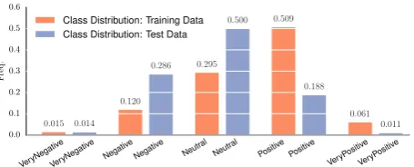
In addition, as shown in Figure1(“Class Distri-bution: Training data”), the classification problem is unbalanced as the distribution of the examples across the five sentiment categories is not uniform. To account for this, I assigned class weights to the examples when training the Logistic Regression. The goal is to penalize more misclassification er-rors in the less frequent classes. The weights are inversely proportional to the number of instances of each class.5 _{This is also motivated by the fact} that the official evaluation measure is the macro-averaged Mean Absolute Error (MAEM) that is

av-eraged across the different classes and accounts for the distance between the true and predicted class. More information about the evaluation met-rics used can be found at (Rosenthal et al.,2017).

3.2 Fine-grained tweet quantification

While the aim of classification is to assign a cate-gory to each tweet, the aim of quantification is to estimate the prevalence of a category to a set of tweets. Several methods for quantification have been proposed: I cite for instance the work of G. Forman on classify and count and probabilistic classify and count (Forman,2008) and the recently proposed ordinal quantification trees (Da San Mar-tino et al.,2016). In this work, I focus on a classify and count approach, which simply requires classi-fying the tweets and then aggregating the classifi-cation results. The official evaluation measure is Earth Movers Distance (EMD) averaged over the

5_{From scikit-learn: ‘LogisticRegression(class weight =}

Subtask C & E

Train2016 5,482

Development2016 1,810 DevTest2016 1,778

Test2016 20,632

Test2017 12,137

Table 1: Size of the data used for training and de-velopment purposes. We only relied on the Se-mEval 2016 datasets.

Subtask C Subtask E

Team Score Team Score

BB twtr 0.4811 BB twtr 0.245 DataStories 0.5552 TwiSe 0.269 Amobee-C-137 0.5993 funSentiment 0.273 Tweester 0.6234 ELiRF-UPV 0.306 TwiSe 0.6400 NRU-HSE 0.317

Table 2: Top-5 systems ranks for Subtask C based on MAEMand of Subtask E based on EMD.

subjects of the data, described in detail at ( Rosen-thal et al.,2017).

The classification and the quantification meth-ods I use rely on efficient operations in terms of memory (hashing) and computational resources (linear models). The feature extraction and learn-ing operations are naturally parallellizable. I be-lieve that this is an important advantage, as the end-to-end system is robust and fast to train. 4 The Experimental Framework

The data Table1shows the data released by the task organizers. To tune the hyper-parameters of my models, I used a simple validation mecha-nism: I concatenated the “Train2016”, “Devel-opment2016”, and “DevTest2016” (9,070 tweets totally) to use them as training and I left the “Test2016” as validation data. I acknowledge that using the “Test2016” part of the data only for val-idation purposes may be limiting in terms of the achieved performance, since these data could have also used to train the system. I also highlight that by using more elaborate validation strategies like using the subjects of the tweets, one should be able to achieve better results for tuning.

Official Rankings Table 2 shows the perfor-mance the systems achieved. There are two main observations. For Subtask C, where TwiSe is ranked 5th_{, I note that the system is a slightly}

improved version of the system of (Balikas and Amini, 2016), ranked first in the Subtask in the 2016 edition. The only difference is the addition

VeryNegativ e

VeryNegativ e

Negativ e

Negativ e

Neutral Neutral Positiv

e Positiv

e

VeryPositiv e

VeryPositiv e

0.0 0.1 0.2 0.3 0.4 0.5 0.6

F

req

.

0.015

0.120

0.295

0.509

0.061 0.014

0.286

0.500

0.188

0.011

Class Distribution: Training Data Class Distribution: Test Data

Figure 1: The distribution of the instances in the training and test sets among the five sentiment classes. The figure is rendered better with color.

of the extra features from clustering the word em-beddings. This entails that significant progress was made to the task, which is either due to the extra data (“Test2016” we only used for valida-tion) or more efficient algorithms. On the other hand, TwiSe is ranked 2nd _{in Subtask E. This,}

along with the simplicity of the approach used that is based on aggregating the counts of the classifi-cation step, entails that there is more work to be done in this direction.

Five-Scale Classification: Error Analysis An-alyzing the classification errors, one finds out that the (macro-averaged) mean-absolute-error per sentiment category is distributed as follows:

VeryNegative: 0.836, Negative: 0.566, Neutral:

0.584, Positive: 0.771, VeryPositive: 0.443. The system performed the best in theVeryPositiveclass (lowest error) and the worst in the VeryNegative

class. Interestingly, the system did not do as well in the Positive class. To better understand why, Figure 1 plots the distribution of the instances across the five sentiment classes, for the training data we used and the test data. Notice how the Positive class is the dominant in the training data, while this changes in the test data. I believe that that the distribution drift, between the training and test data is indicative as of why the system per-formed poorly in the “Positive” class.

and “medicaid”, which are both skewed towards the negative sentiment, are 1.328 and 0.896 re-spectively. Although a more detailed error analy-sis is required in order to improve the performance of the system, I believe that the distribution drift between the training examples and the examples of a subject plays an important role. This may be further enhanced by the fact I used a classify and count approach which does not account for drifts. 5 Conclusion

The paper described the participation of TwiSe

in the subtasks C and E of of the “Twitter Sen-timent Evaluation” Task of SemEval-2017. Im-portantly, my system was ranked 2nd _{in Subtask}

E, “Five-point Sentiment Quantification” using a simple classify and count approach on top of a Lo-gistic Regression. An interesting future work di-rection towards improving the system aims at bet-ter handling distribution drifts between the train-ing and test data.

References

David Arthur and Sergei Vassilvitskii. 2007.

k-means++: The advantages of careful seeding. In

Proceedings of the eighteenth annual ACM-SIAM symposium on Discrete algorithms. Society for In-dustrial and Applied Mathematics, pages 1027– 1035.

Georgios Balikas and Massih-Reza Amini. 2016. Twise at semeval-2016 task 4: Twitter sentiment

classification. InSemEval@NAACL-HLT 2016, San

Diego, CA, USA, June 16-17, 2016. pages 85–91. Steven Bird, Ewan Klein, and Edward Loper.

2009. Natural Language Processing with Python.

O’Reilly Media.

Richard H. Byrd, Peihuang Lu, Jorge Nocedal, and Ciyou Zhu. 1995. A limited memory algorithm for

bound constrained optimization. SIAM J. Scientific

Computing16(5):1190–1208.

Giovanni Da San Martino, Wei Gao, and Fabrizio

Se-bastiani. 2016. Ordinal text quantification. In

Pro-ceedings of the 39th International ACM SIGIR con-ference on Research and Development in Informa-tion Retrieval. ACM, pages 937–940.

George Forman. 2008. Quantifying counts and costs

via classification. Data Mining and Knowledge

Dis-covery17(2):164–206.

Kevin Gimpel, Nathan Schneider, Brendan O’Connor, Dipanjan Das, Daniel Mills, Jacob Eisenstein, Michael Heilman, Dani Yogatama, Jeffrey Flanigan, and Noah A Smith. 2011. Part-of-speech tagging

for twitter: Annotation, features, and experiments. In Proceedings of the 49th Annual Meeting of the Association for Computational Linguistics: Human Language Technologies: short papers-Volume 2. As-sociation for Computational Linguistics, pages 42– 47.

Alec Go, Richa Bhayani, and Lei Huang. 2009. Twit-ter sentiment classification using distant supervision.

CS224N Project Report, Stanford1:12.

Minqing Hu and Bing Liu. 2004. Mining and

summa-rizing customer reviews. InProceedings of the tenth

ACM SIGKDD international conference on Knowl-edge discovery and data mining. ACM, pages 168– 177.

Svetlana Kiritchenko, Xiaodan Zhu, and Saif M Mo-hammad. 2014. Sentiment analysis of short

infor-mal texts. Journal of Artificial Intelligence Research

pages 723–762.

Tomas Mikolov, Kai Chen, Greg Corrado, and Jeffrey Dean. 2013. Efficient estimation of word

represen-tations in vector space.CoRRabs/1301.3781.

Saif M Mohammad and Peter D Turney. 2010. Emo-tions evoked by common words and phrases: Us-ing mechanical turk to create an emotion lexicon. In Proceedings of the NAACL HLT 2010 workshop on computational approaches to analysis and gen-eration of emotion in text. Association for Computa-tional Linguistics, pages 26–34.

Ioannis Partalas, C´edric Lopez, Nadia Derbas, and Ruslan Kalitvianski. 2016. Learning to search for

recognizing named entities in twitter. WNUT 2016

page 171.

F. Pedregosa, G. Varoquaux, A. Gramfort, V. Michel, B. Thirion, O. Grisel, M. Blondel, P. Pretten-hofer, R. Weiss, V. Dubourg, J. Vanderplas, A. Pas-sos, D. Cournapeau, M. Brucher, M. Perrot, and E. Duchesnay. 2011. Scikit-learn: Machine learning

in Python. Journal of Machine Learning Research

12:2825–2830.

Sara Rosenthal, Noura Farra, and Preslav Nakov. 2017. SemEval-2017 task 4: Sentiment analysis in

Twit-ter. InProceedings of the 11th International

Work-shop on Semantic Evaluation. Association for Com-putational Linguistics, Vancouver, Canada, SemEval ’17.

Kilian Weinberger, Anirban Dasgupta, John Langford, Alex Smola, and Josh Attenberg. 2009. Feature

hashing for large scale multitask learning. In

Pro-ceedings of the 26th Annual International Confer-ence on Machine Learning. ACM, pages 1113– 1120.

Theresa Wilson, Janyce Wiebe, and Paul Hoffmann. 2005. Recognizing contextual polarity in

phrase-level sentiment analysis. InProceedings of the