Incorporating visual features into word embeddings: A bimodal autoencoder based approach

Incorporating visual features into word embeddings:

A bimodal autoencoder-based approach

Mika Hasegawa Waseda University [email protected]

Tetsunori Kobayashi Waseda University

[email protected]

Yoshihiko Hayashi Waseda University [email protected]

Abstract

Multimodal semantic representation is an evolving area of research in natural language process-ing as well as computer vision. Combinprocess-ing or integratprocess-ing perceptual information, such as visual features, with linguistic features is recently being actively studied. This paper presents a novel bi-modal autoencoder model for multibi-modal representation learning: the autoencoder learns in order to enhance linguistic feature vectors by incorporating the corresponding visual features. During the runtime, owing to the trained neural network, visually enhanced multimodal representations can be achieved even for words for which direct visual-linguistic correspondences are not learned. The em-pirical results obtained with standard semantic relatedness tasks demonstrate that our approach is generally promising. We further investigate the potential efficacy of the enhanced word embeddings in discriminating antonyms and synonyms from vaguely related words.

1

Introduction

The efficient learning and the effective exploitation of a distributed representation of words, phrases, and sentences are active research topics in NLP (Bengio et al., 2013; Mikolov et al., 2013). Theoretically sup-ported by the concept of grounded cognition (Barsalou, 2008) and technically endorsed by the progress of deep learning techniques, this line of research has been further pursued in order to incorporate percep-tual information, such as visual features, into linguistic embeddings (Silberer and Lapata, 2014; Bruni et al., 2014; Kiela and Bottou, 2014; Kiela et al., 2016). The resulting semantic representation is often referred to asmultimodal semantic representation.

Two fundamental requirements, however, may not have been fulfilled simultaneously: (1) the zero-shot representation learningof words, and (2) the exploitation of existing useful resources. It should be noted that zero-shot representation learning in the context of the present research means a computational process for obtaining an appropriate multimodal representation even for a word for which direct visual-linguistic correspondences have not been learned. In this paper, a bimodal autoencoder1model, named ViEW (visually enhanced word embeddings), is proposed for incorporating visual features into existing word embeddings.

This architecture facilitates bimodal representation learning from the given visual-linguistic corre-spondences. In the training, the autoencoder learns to reproduce a linguistic word embedding vector, while having an additional input vector (of the same dimensionality) that represents the corresponding visual features. During the runtime, by exploiting the trained neural network parameters, the autoencoder can construct a visually enhanced word embedding even for a word for which direct visual-linguistic cor-respondences have not been learned. It should be noted here that these visual and linguistic features could be drawn from independently developed existing resources.

The experimental results demonstrate that our model exhibits state-of-the-art performances in stan-dard semantic relatedness tasks, some of which innately contain zero-shot instances. We further discuss

1_{Autoencoders are generally used in representation learning; after training, the compact representation of an input data can}

the potential efficacy of the enhanced word embeddings in discriminating antonyms and synonyms from vaguely related words.

2

Related work

The approaches to multimodal representation learning can be primarily classified by the method of in-formation fusion or integration. In addition, so-calledzero-shot representation learningis an important factor for characterizing an approach.

Among the several researches on multimodal semantic representation, only two of them are summa-rized here. Bruni et al. (2014) applied singular value decomposition (SVD) to a word-feature matrix, where each word is represented by the concatenation of a linguistic vector and the corresponding visual vector. The linguistic vectors are generated using the Strudel method (Baroni et al., 2010), and the vi-sual vectors are obtained by applying a conventional feature-extraction method that relies on the local features of bag-of-visual-words (BoVW). Kiela and Bottou (2014) simply used vector concatenation, in which the visual features were extracted from a convolutional neural network (CNN), and the linguistic features were Word2Vec (Mikolov et al., 2013) word embeddings. These works pioneered this research direction by developing methods to combine or integrate linguistic and visual features; however, they suffered from the inability to handle zero-shot representation learning.

Zero-shot representation learning, in the context of the present research, indicates a computational process for achieving an appropriate multimodal representation even for a word for which direct visual-linguistic correspondences have not been learned. This concept may have originated in the field of computer vision (Lampert and Harmeling, 2009) and has been a continuously active research topic. It is crucial in computer vision and other research areas as well, given a potential situation in which sufficient annotations for all possible categories or concepts cannot be expected.

In order to tackle the zero-shot learning problem in the context of multimodal representation learning, Lazaridou et al. (2015) proposed the multimodal skip-gram (MMSG) model that extends the original skip-gram model (Mikolov et al., 2013) by incorporating visual features. More specifically, a restricted set of words in the training text corpus is accompanied with the corresponding images, and the model builds word vectors by learning to jointly predict linguistic and visual features. The joint objective enables the propagation of visual information to representations of words for which no direct visual evidence is available in the training, and hence, the model can realize zero-shot image labeling and retrieval. However, it should be noted that this framework requires a joint learning process, which means that independently developed existing linguistic or visual features cannot be used.

As in (Lazaridou et al., 2015), our ViEW model addresses the zero-shot representation learning problem but does not adopt a joint-learning approach. This allows us to fully exploit the existing inde-pendently developed linguistic and visual resources. The heart of the proposed approach is a bimodal autoencoder that integrates bimodal inputs by maintaining a specially designed loss function that is de-scribed afterward. It should be mentioned here that Silberer and Lapata (2014) have already adopted a similar architecture (in a sense). Their architecture, however, integrates modality-dependent autoen-coders in a hidden layer, which means that the multimodal representations can only be built for pairs of visual and linguistic inputs. This means that the autoencoder cannot cope with zero-shot representation learning. Recently, a literature (Kodirov et al., 2017) that proposed an autoencoder architecture for zero-shot learning was published in a computer vision conference. Although the architecture is apparently similar to our ViEW model, their primary input/output is a visual feature instead of a linguistic feature.

3

ViEW model

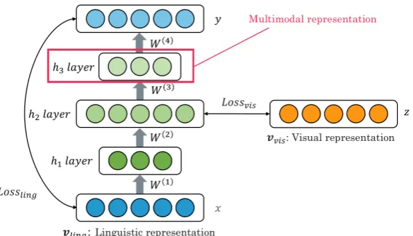
Figure 1: Architecture of the ViEW model.

between the linguistic input and the visual input (Lossvis). The rationale behind the architecture is that

if a pair of linguistic features are similar, the corresponding visual feature vectors would also be similar. We can expect that a visually enhanced representation could be obtained from the hidden layers (shown in green), even for a word for which direct visual-linguistic correspondences have not been learned.

In particular, during the training time, two losses (Lling andLvis) are simultaneously optimized in

order to minimize the mean square errors (MSEs).Llingmeasures the error between the input and output

linguistic representations, whereasLvisindicates the error between the visual and the hidden-layer (h2)

representations.

L = δlingLling+δvisLvis (1)

Lling = n

∑

k=1

(

x(k)−y(k) )2

(2)

Lvis = n

∑

k=1

(

h(k)₂ −z(k) )2

= n

∑

k=1

(

(tanh(W(2)x1+b(2)))(k)−z(k)

)2

(3)

xn = tanh

(

W(n)xn−1+b(n)

)

(4)

In the formulation, x = {x(1), ..., x(n)} andy = {y(1), ..., y(n)},∈ Rdling×n_{denote the sequences of}

linguistic input and output representations respectively; z = {z(1), ...z(n)} ∈ Rdvis×n _{represents the}

sequence of visual representations, andnis the number of trained word–image pairs. In addition,δling

andδvisare hyper-parameters that balance the linguistic and visual components2.

During the runtime, only a linguistic representation (word-embedding vector) is fed into the network, and the network performs a forward computation by employing the trained parameters. We adopt the h3-layer vectors, rather than the h2-h3-layer vectors as the multimodal semantic representation. This decision was made because the h2-layer vectors might be too influenced by visual features, whereas the h3-layer vectors could more mildly incorporate the visual features3, and hence, they are more suitable as a semantic representation that can be used in a variety of linguistic semantic tasks.

It should be mentioned that the dimensionalities of the h2-layer vector and visual feature vector must be identical, as we compute the MSE between them. In order to maintain this constraint, we have experimented with several methods for reducing the dimensionality of the visual feature vector (described in section 4.3.2).

2

In the experiments, we adopted equal weights that were determined after a rough parameter search.

3

4

Experimental setup

4.1 Task and the evaluation measure

We evaluate the performance of the achieved multimodal representations using standard semantic relat-edness tasks (Gabrilovich and Markovitch, 2007; Budanitsky and Hirst, 2006), which would enable us to compare our results with that of previous works. As semantic relatedness covers a wider range of lexical or semantic relationships between words than semantic similarity, the relatedness tasks may be more suitable for assessing the performance of multimodal semantic representations, which would encode our implicit perceptual knowledge. We mainly employ the MEN (Bruni et al., 2014) dataset and assess the performance by measuring the Spearman’s rank correlation coefficients between the MEN’s gold ratings and the predicted relatedness.

4.2 Test dataset

The MEN dataset was specifically developed for evaluating multimodal semantic models (Bruni et al., 2014). In addition, we used the SimLex-999 (Hill et al., 2015) and the SemSim/VisSim (Silberer and Lapata, 2014) datasets to further investigate the applicability of the proposed model in other datasets having different characteristics.

• MEN: This dataset includes 3,000 word pairs created from 751 distinct words. Each pair in the dataset was given a semantic relatedness score in the range of [0, 1]. It contains highly semantically related pairs (e.g.,beach/sandrated as 0.96) as well as low-scored pairs (e.g.,bakery/zebrarated as 0). Each word in the dataset was assigned a part of speech (POS) tag: verb, adjective, or noun.

• SimLex-999: This is a dataset of 999 word pairs that is used for assessing the ability of a semantic model in capturing semantic similarity, rather than semantic relatedness or association. As the au-thors argue and several empirical results suggest, this dataset poses challenges to the most models based on the distributional hypothesis.

• SemSim/VisSim: This is a dataset of 7,576 word pairs, each of which is annotated using not only semantic similarities (SemSim) but also visual similarities (VisSim), so that the user can compare the performances of her/his model in predicting different types of similarities.

4.3 Features

As described in section 3, our ViEW model can consume existing visual and linguistic features. In the experiments, we prepared both these types of features as detailed below. It should be noted that these processes are completely independent from the construction and application of the ViEW model.

4.3.1 Linguistic features

We extracted 300-dimensional word embeddings by applying the skip-gram model (Mikolov et al., 2013). The text corpus used was enwiki94, which consisted of a collection of the first 109 _{bytes of}

text from the Wikipedia 2009 dump. We adopted the following hyper-parameters: the window size was set as five, and the frequency threshold for inclusion was five.

4.3.2 Visual features

In order to obtain the visual representation of a word, GoogLeNet (Szegedy et al., 2015) was used to analyze the corresponding images and derive the visual feature vector. GoogLeNet is well known owing to its deep neural network structure and its superior performance, which was demonstrated in the ImageNet Large Scale Visual Recognition Competition (ILSVRC2014). Kiela et al. (2016) states that GoogLeNet balances its performance and memory-efficiency. We constructed a 1024-dimensional

visual feature vector for a word by averaging the resulting hidden-layer vectors obtained from the 50–100 corresponding images. As the source of the images, we used the following image datasets. Their utility and problems were examined in the experiments.

• ImageNet (Krizhevsky et al., 2012)5: It is a collection of 14 million high-quality images assigned to 21K WordNet synsets. Generally, the target object associated with a synset is depicted at the center of an image, which means that the obtained visual feature chiefly represents the target concept. Therefore, the images are clean but the dataset only contains images associated with concrete concepts.

• ESP-Game dataset (von Ahn and Dabbish, 2004)6: It contains 100K images, each of which has multiple labels assigned through “game with a purpose.” This means that (1) the object associated with an image label is not necessarily the primary visual component in the image, and (2) an image label does not always have a corresponding visual object in the image. Thus, the images in the ESP-Game dataset are obviously noisier (in terms of target word) as compared to the ImageNet images. However, it is expected that this dataset may provide useful visual co-occurrence information in some cases. Furthermore, it should be noted that the images are associated not only with concrete nouns but also with adjectives and verbs.

Dimensionality reduction: As mentioned in section 3, the dimensionality of an h2-layer vector and that of the visual feature vector must be identical. This means that if we require a 300-dimensional h2-layer vector, the corresponding 1024-dimensional visual feature vector extracted from a CNN hidden layer must be reduced in order to match its dimensionality. In order to perform this task, we have applied two methods: the use of a principal component analysis (PCA) and that of an autoencoder (AE). The results obtained on using these two methods were compared with those obtained in the case of no dimensionality reduction (RAW setting). In the RAW setting, the dimensionality of the h2-layer vector was 1024 rather than 300, which implies that the multimodal representations might be sparse.

5

Results and discussion

5.1 Results: non-zero-shot settings

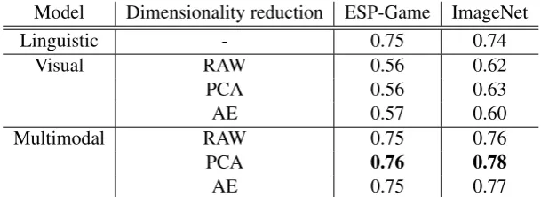
Although the zero-shot representation learning is the main focus of the present work, the efficacy of the proposed model should primarily be evaluated in a setting in which all the words in a test dataset have undergone the bimodal training process. This setting is henceforth referred to as “non-ZS.” Table 1 displays the overall results for the non-ZS setting for which a portion of the MEN dataset was employed. The size of the portion used varies depending on the coverage of the images in the exploited image source. Around 23% and 42% of the words in the MEN dataset were accompanied with the corresponding images with the ESP-Game and ImageNet, respectively. The table also compares the following models: linguistic, visual, and multimodal; the multimodal models are further classified by the method used for the dimensionality reduction of the visual features.

Table 1 demonstrates that the multimodal representation enabled by the ViEW model is superior to that of the unimodal models. It also shows that ImageNet yielded better results, thus demonstrating the superiority of this image source. However, interestingly, the ViEW model seems to compensate for the problems with the ESP-Game image source well: the difference in the Spearman coefficient between the two image sources is smaller in the case of the MM as compared to the visual unimodal model. It should be further noted that PCA was a better method for visual feature dimensionality reduction, particularly in this setting.

Table 2 compares our results with those of related works, showing that the ViEW model (with PCA dimensionality reduction) almost achieves state-of-the-art performances.

5

http://image-net.org

Model Dimensionality reduction ESP-Game ImageNet

Linguistic - 0.75 0.74

Visual RAW 0.56 0.62

PCA 0.56 0.63

AE 0.57 0.60

Multimodal RAW 0.75 0.76

PCA 0.76 0.78

AE 0.75 0.77

Table 1: ViEW model results for the non-ZS setting (MEN dataset).

Model ESP-Game ImageNet ViEW (PCA) 0.76 0.78

Kiela and Bottou (2014) 0.72 0.70 Bruni et al. (2014) 0.78 -Lazaridou et al. (2015): MMSG-A - 0.74 Lazaridou et al. (2015): MMSG-B - 0.76

Table 2: Comparison of the non-ZS results (MEN dataset).

5.2 Results: zero-shot including settings

Table 3 summarizes the results for the settings for which the entire test dataset is used. We refer to this setting as “ZS,” because it inherently includes words without the corresponding trained images (zero-shot conditions). As shown in the table, the ViEW model exhibited a superior performance with the MEN dataset, which is our primary dataset. In contrast, the MMSG models (A and MMSG-B) (Lazaridou et al., 2015) achieved better results with the other datasets, such as SimLex-999, SemSim, and VisSim, which indicates that there exist issues to be further explored with the ViEW model.

Model MEN (100%) SimLex-999 (100%) SemSim (100%) VisSim (100%)

ViEW (PCA) 0.76 0.34 0.68 0.55

MMSG-A 0.75 0.37 0.72 0.63

MMSG-B 0.74 0.40 0.66 0.60

Table 3: Comparison of the ZS results with four datasets.

5.3 Results: POS breakdown

Noun (2005 pairs) Adjective (96 pairs) Verb (29 pairs) Model ZS non-ZS (21%) ZS non-ZS (66%) ZS non-ZS (31%)

Ling. 0.75 0.76 0.60 0.44 0.37 0.78

Vis. - 0.57 - 0.64 - -0.20

MM RAW 0.75 0.77 0.64 0.53 0.37 0.78 PCA 0.76 0.78 0.64 0.54 0.38 0.73 AE 0.75 0.77 0.63 0.53 0.36 0.73

Table 4: POS breakdown of the MEN dataset results (Image source: ESP-Game).

5.4 Discussion: antonyms and synonyms

It is often argued that text-based distributional/distributed representations hardly distinguish synonyms from other semantically related words. This is natural because these approaches rely heavily on con-textual similarities. One of these typical relation types is antonymy: antonyms are frequently predicted as highly similar or related. In this subsection, we examine the potential efficacy of the multimodal representation in discriminating antonyms and synonyms from vaguely related words.

Among the pairs of antonymous adjectives defined in WordNet, we could assign the ViEW multi-modal representations to 4,172 pairs by employing ImageNet as the image source. Table 5 shows the examples ofk-neighbor words retrieved for some adjectives: “rural,” “cold,” and “happy.” Similarly, we assigned multimodal representations to 106,472 synonymous noun pairs.

Word MM (ImageNet) MM (ESP-Game) Ling.

rural countryside, urbanised,homesteads countryside,heckmondwike, urbanised urban,exurban,urbanizing farmers, urban crofting,smalandian suburban,countryside

cold freeze, warmed, smothered freezing,thawing,cool bloodedness, warm freezing, grit bloodedness,colder warmed,clammy,cool

happy newlyweds, darlin,glad cheerful,glad, sentimental doggone,happier, bummed merrily, wistful waifs, goodnight derkins, hooky

Table 5: Comparison ofk-neighbor words (k= 5) for some adjectives.

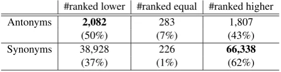
By using the Word2Vec word embedding vectors and multimodal vectors, we compared the similarity ranks obtained for these representations. As summarized in Table 6, some of the antonymous pairs had low ranks, and several of the synonymous pairs were ranked relatively higher, which is promising. These results may imply the potential efficacy of the multimodal representation in propagating visual information even to visually novel words and in filtering semantically related but perceptually irrelevant words or concepts.

#ranked lower #ranked equal #ranked higher Antonyms 2,082 283 1,807

(50%) (7%) (43%)

Synonyms 38,928 226 66,338

(37%) (1%) (62%)

Table 6: Changes in the similarity ranks of antonyms/synonyms (ImageNet).

5.5 Discussion: comparison of the image sources

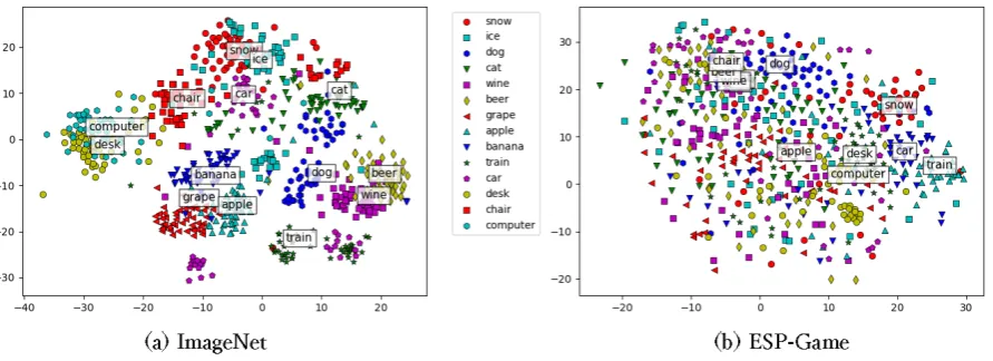
survey, and the paper concluded that “The ESP Game dataset does not appear to work very well and is best avoided. If we have the right coverage, then ImageNet gives good results, ...” In order to visually compare the nature of the visual features obtained respectively from ImageNet and ESP-Game, Figure 2 displays two-dimensional visualizations of the obtained vectors. t-SNE (Maaten and Hinton, 2008) was applied in the visualization. Each of the labels in these figures represents the centroid of a target word. On comparing these figures, it is observed that the centroids for semantically related words are relatively closely located in both cases, but the dispersion is more evident for the features obtained from the ESP-Game dataset. These differences may be attributed to the difference in the nature of the datasets as discussed in the previous section. That is, the images in ImageNet are clean in terms of the depiction of a target concept, whereas ESP-Game images are generally noisy.

Figure 2: t-SNE visualization of image features.

This insight was already confirmed by the results of our experiments. However, the differences in performance (Spearman coefficients) were not very significant as expected, particularly when employed with the multimodal models. This may be partly attributed to the nature of the ESP-Game dataset: visual co-occurrences would have been captured relatively well, and this might have contributed to enhancing the linguistic representations, which form the basis of the multimodal representations.

6

Concluding remarks

This paper presented a novel bimodal autoencoder model for incorporating visual features into existing word embeddings. Although the empirical results were generally promising, there is still room for im-provement and exploration. We would like to incorporate more features, such as POS, semantic class, and abstractness/correctness (Kiela et al., 2014), into the neural network structure. We intend to develop a method for extracting effective features in order to capturedynamicsfrom videos; this may be vital in representing the visual meaning of motion verbs and the like. Another potential research direction could involve the evaluation of the utility of multimodal representations in downstream applications, such as cross-modal mapping/retrieval.

Acknowledgment

References

Baroni, M., B. Murphy, E. Barbu, and M. Poesio (2010). Strudel: A corpus-based semantic model based on properties and types. Cogn. Sci. 34(2), 222–254.

Barsalou, L. W. (2008). Grounded cognition. Annu. Rev. Psychol. 59(August), 617–645.

Bengio, Y., A. Courville, and P. Vincent (2013). Representation Learning : A Review and New Perspec-tives. IEEE Trans. Pattern Anal. Mach. Intell. 35, 1798—-1828.

Bruni, E., D. Gatica-perez, N. K. Tran, and M. Baroni (2014). Multimodal distributional semantics. J. Artif. Intell. Res. 49(December), 1–47.

Budanitsky, A. and G. Hirst (2006). Evaluating WordNet-based Measures of Lexical Semantic Related-ness. Comput. Linguist. 32(1), 13–47.

Gabrilovich, E. and S. Markovitch (2007). Computing semantic relatedness using wikipedia-based ex-plicit semantic analysis.IJCAI Int. Jt. Conf. Artif. Intell., 1606–1611.

Hill, F., R. Reichart, and A. Korhonen (2015). SimLex-999: Evaluating Semantic Models with (Genuine) Similarity Estimation.Comput. Linguist. 41(4), 665–695.

Kiela, D. and L. Bottou (2014). Learning Image Embeddings using Convolutional Neural Networks for Improved Multi-Modal Semantics. EMNLP 2014, 36–45.

Kiela, D., S. Clark, A. L. Ver, S. Clark, M. Baroni, B. Murphy, E. Barbu, and M. Poesio (2016). Compar-ing Data Sources and Architectures for Deep Visual Representation LearnCompar-ing in Semantics. EMNLP 2016 34(2), 447–456.

Kiela, D., F. Hill, A. Korhonen, and S. Clark (2014). Improving Multi-Modal Representations Using Image Dispersion : Why Less is Sometimes More.ACL 2014.

Kodirov, E., T. Xiang, S. Gong, and Q. Mary (2017). Semantic Autoencoder for Zero-Shot Learning.

IEEE Conf. Comput. Vis. Pattern Recognit., 3174–3183.

Krizhevsky, A., I. Sutskever, and G. E. Hinton (2012). ImageNet Classification with Deep Convolutional Neural Networks. Adv. Neural Inf. Process. Syst., 1–9.

Lampert, C. H. and S. Harmeling (2009). Learning To Detect Unseen Object Classes by Between-Class Attribute Transfer.IEEE Conf. Comput. Vis. Pattern Recognit..

Lazaridou, A., T. P. Nghia, and M. Baroni (2015). Combining Language and Vision with a Multimodal Skip-gram Model. NAACL 2015, 153–163.

Maaten, L. V. D. and G. Hinton (2008). Visualizing Data using t-SNE. J. Mach. Learn. Res. 9, 2579– 2605.

Mikolov, T., I. Sutskever, K. Chen, G. Corrado, and J. Dean (2013). Distributed Representations of Words and Phrases and their Compositionality.Proc. NIPS 9, 1–9.

Silberer, C. and M. Lapata (2014). Learning Grounded Meaning Representations with Autoencoders.

Proc. 52nd Annu. Meet. Assoc. Comput. Linguist. (Volume 1 Long Pap., 721–732.

Szegedy, C., W. Liu, Y. Jia, P. Sermanet, S. Reed, D. Anguelov, D. Erhan, V. Vanhoucke, and A. Rabi-novich (2015). Going deeper with convolutions.Proc. IEEE Comput. Soc. Conf. Comput. Vis. Pattern Recognit. 07-12-June, 1–9.