Proceedings of the Human Language Technology Conference of the North American Chapter of the ACL, pages 104–111,
Alignment by Agreement
Percy Liang
UC Berkeley Berkeley, CA 94720 [email protected]
Ben Taskar
UC Berkeley Berkeley, CA 94720 [email protected]
Dan Klein
UC Berkeley Berkeley, CA 94720 [email protected]
Abstract
We present an unsupervised approach to symmetric word alignment in which two simple asymmetric models are trained jointly to maximize a combination of data likelihood and agreement between the models. Compared to the stan-dard practice of intersecting predictions of independently-trained models, joint train-ing provides a 32% reduction in AER. Moreover, a simple and efficient pair of HMM aligners provides a 29% reduction in AER over symmetrized IBM model 4 predictions.
1 Introduction
Word alignment is an important component of a complete statistical machine translation pipeline (Koehn et al., 2003). The classic approaches to un-supervised word alignment are based on IBM mod-els 1–5 (Brown et al., 1994) and the HMM model (Ney and Vogel, 1996) (see Och and Ney (2003) for a systematic comparison). One can classify these six models into two groups: sequence-based models (models 1, 2, and HMM) and fertility-based models (models 3, 4, and 5).1 Whereas the sequence-based models are tractable and easily implemented, the more accurate fertility-based models are intractable and thus require approximation methods which are
1
IBM models 1 and 2 are considered sequence-based models because they are special cases of HMMs with transitions that do not depend on previous states.
difficult to implement. As a result, many practition-ers use the complex GIZA++ software package (Och and Ney, 2003) as a black box, selecting model 4 as a good compromise between alignment quality and efficiency.
Even though the fertility-based models are more accurate, there are several reasons to consider av-enues for improvement based on the simpler and faster sequence-based models. First, even with the highly optimized implementations in GIZA++, models 3 and above are still very slow to train. Sec-ond, we seem to have hit a point of diminishing re-turns with extensions to the fertility-based models. For example, gains from the new model 6 of Och and Ney (2003) are modest. When models are too complex to reimplement, the barrier to improvement is raised even higher. Finally, the fertility-based models are asymmetric, and symmetrization is com-monly employed to improve alignment quality by intersecting alignments induced in each translation direction. It is therefore natural to explore models which are designed from the start with symmetry in mind.
In this paper, we introduce a new method for word alignment that addresses the three issues above. Our development is motivated by the observation that in-tersecting the predictions of two directional models outperforms each model alone. Viewing intersec-tion as a way of finding predicintersec-tions that both models agree on, we take the agreement idea one step fur-ther. The central idea of our approach is to not only make the predictions of the models agree at test time, but also encourage agreement during training. We define an intuitive objective function which
porates both data likelihood and a measure of agree-ment between models. Then we derive an EM-like algorithm to maximize this objective function. Be-cause the E-step is intractable in our case, we use a heuristic approximation which nonetheless works well in practice.
By jointly training two simple HMM models, we obtain 4.9% AER on the standard English-French Hansards task. To our knowledge, this is the lowest published unsupervised AER result, and it is com-petitive with supervised approaches. Furthermore, our approach is very practical: it is no harder to implement than a standard HMM model, and joint training is no slower than the standard training of two HMM models. Finally, we show that word alignments from our system can be used in a phrase-based translation system to modestly improve BLEU score.
2 Alignment models: IBM 1, 2 and HMM
We briefly review the sequence-based word align-ment models (Brown et al., 1994; Och and Ney, 2003) and describe some of the choices in our implementation. All three models are generative models of the form p(f | e) = P
ap(a,f | e), where e = (e1, . . . , eI) is the English sentence, f = (f1, . . . , fJ) is the French sentence, and a = (a1, . . . , aJ) is the (asymmetric) alignment which
specifies the position of an English word aligned to each French word. All three models factor in the following way:
p(a,f |e) = J
Y
j=1
pd(aj |aj−, j)pt(fj |eaj), (1)
wherej−is the position of the last non-null-aligned French word before positionj.2
The translation parameters pt(fj | eaj) are pa-rameterized by an (unsmoothed) lookup table that stores the appropriate local conditional probability distributions. The distortion parameterspd(aj =i0 | aj− = i) depend on the particular model (we write aj = 0to denote the event that thej-th French word
2
The dependence onaj− can in fact be implemented as a first-order HMM (see Och and Ney (2003)).
is null-aligned):
pd(aj= 0|aj−=i) = p0
pd(aj=i0 = 06 |aj−=i) ∝
(1−p0)·
1 (IBM 1)
c(i0−bjI
Jc) (IBM 2) c(i0−i) (HMM),
wherep0 is the null-word probability and c(·) con-tains the distortion parameters for each offset argu-ment. We set the null-word probability p0 = I+11 depending on the length of the English sentence, which we found to be more effective than using a constantp0.
In model 1, the distortionpd(· | ·)specifies a
uni-form distribution over English positions. In model
2,pd(· | ·)is still independent ofaj−, but it can now
depend onjandi0throughc(·). In the HMM model, there is a dependence onaj− =i, but only through c(i−i0).
We parameterize the distortionc(·)using a multi-nomial distribution over 11 offset buckets c(≤ −5), c(−4), . . . , c(4), c(≥5).3 We use three sets of distortion parameters, one for transitioning into the first state, one for transitioning out of the last state, and one for all other transitions. This works better than using a single set of parameters or ignoring the transitions at the two ends.
3 Training by agreement
To motivate our joint training approach, we first consider the standard practice of intersecting align-ments. While the English and French sentences play a symmetric role in the word alignment task, sequence-based models are asymmetric: they are generative models of the formp(f | e) (E→F), or p(e|f)(F→E) by reversing the roles of source and
target. In general, intersecting the alignment predic-tions of two independently-trained directional mod-els reduces AER, e.g., from 11% to 7% for HMM models (Table 2). This suggests that two models make different types of errors that can be eliminated upon intersection. Figure 1 (top) shows a common type of error that intersection can partly remedy. In
3
In d ep en d en t tr ai n in g w e d e e m e
d it
i n a d v i s a b l
e to
a t t e n d t h e m e e t i n g a n
d so
i n f o r m e d c o j o . nous ne avons pas cru bon de assister ` a la r´eunion et en avons inform´e le cojo en cons´equence . w e d e e m e
d it
i n a d v i s a b l
e to
a t t e n d t h e m e e t i n g a n
d so
i n f o r m e d c o j o . nous ne avons pas cru bon de assister ` a la r´eunion et en avons inform´e le cojo en cons´equence . w e d e e m e
d it
i n a d v i s a b l
e to
a t t e n d t h e m e e t i n g a n
d so
i n f o r m e d c o j o . nous ne avons pas cru bon de assister ` a la r´eunion et en avons inform´e le cojo en cons´equence .
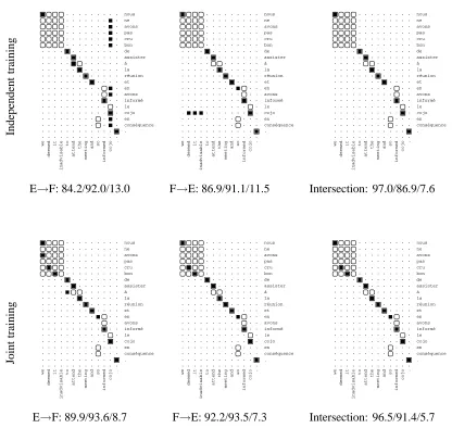
E→F: 84.2/92.0/13.0 F→E: 86.9/91.1/11.5 Intersection: 97.0/86.9/7.6
Jo in t tr ai n in g w e d e e m e d i t i n a d v i s a b l e t o a t t e n d t h e m e e t i n g a n d s o i n f o r m e d c o j o . nous ne avons pas cru bon de assister ` a la r´eunion et en avons inform´e le cojo en cons´equence . w e d e e m e d i t i n a d v i s a b l e t o a t t e n d t h e m e e t i n g a n d s o i n f o r m e d c o j o . nous ne avons pas cru bon de assister ` a la r´eunion et en avons inform´e le cojo en cons´equence . w e d e e m e d i t i n a d v i s a b l e t o a t t e n d t h e m e e t i n g a n d s o i n f o r m e d c o j o . nous ne avons pas cru bon de assister ` a la r´eunion et en avons inform´e le cojo en cons´equence .
[image:3.612.103.519.87.481.2]E→F: 89.9/93.6/8.7 F→E: 92.2/93.5/7.3 Intersection: 96.5/91.4/5.7
Figure 1: An example of the Viterbi output of a pair of independently trained HMMs (top) and a pair of jointly trained HMMs (bottom), both trained on 1.1 million sentences. Rounded boxes denote possible alignments, square boxes are sure alignments, and solid boxes are model predictions. For each model, the overall Precision/Recall/AER on the development set is given. See Section 4 for details.
this example, COJO is a rare word that becomes a garbage collector (Moore, 2004) for the models in both directions. Intersection eliminates the spurious alignments, but at the expense of recall.
Intersection after training produces alignments that both models agree on. The joint training pro-cedure we describe below builds on this idea by en-couraging the models to agree during training. Con-sider the output of the jointly trained HMMs in Fig-ure 1 (bottom). The garbage-collecting rare word is
no longer a problem. Not only are the individual E→F and F→E jointly-trained models better than their independently-trained counterparts, the jointly-trained intersected model also provides a signifi-cant overall gain over the independently-trained in-tersected model. We maintain both high precision and recall.
alignment spaces. We first replace the asymmetric alignments a with a set of indicator variables for
each potential alignment edge (i, j): z = {zij ∈
{0,1} : 1 ≤ i ≤ I,1 ≤ j ≤ J}. Each zcan be
thought of as an element in the set of generalized
alignments, where any subset of word pairs may be
aligned (Och and Ney, 2003). Sequence-based mod-elsp(a |e,f) induce a distribution overp(z |e,f)
by letting p(z | e,f) = 0 for any z that does not
correspond to anya(i.e., ifzcontains many-to-one
alignments).
We also introduce the more compact notation
x = (e,f) to denote an input sentence pair. We
put arbitrary distributions p(e) and p(f)to remove
the conditioning, noting that this has no effect on the optimization problem in the next section. We can now think of the two directional sequence-based models as each inducing a distribution over the same space of sentence pairs and alignments(x,z):
p1(x,z;θ1) =p(e)p(a,f |e;θ1)
p2(x,z;θ2) =p(f)p(a,e|f;θ2).
3.1 A joint objective
In the next two sections, we describe how to jointly train the two models using an EM-like algorithm. We emphasize that this technique is quite general and can be applied in many different situations where we want to couple two tractable models over inputxand outputz.
To train two models p1(x,z;θ1) and p2(x,z;θ2) independently, we maximize the data likelihood Q
xpk(x;θk) = Q
x P
zpk(x,z;θk)of each model separately,k∈ {1,2}:
max θ1,θ2
X
x
[logp1(x;θ1) + logp2(x;θ2)]. (2)
Above, the summation over xenumerates the
sen-tence pairs in the training data.
There are many possible ways to quantify agree-ment between two models. We chose a particularly simple and mathematically convenient measure — the probability that the alignments produced by the two models agree on an examplex:
X
z
p1(z|x;θ1)p2(z|x;θ2).
We add the (log) probability of agreement to the standard log-likelihood objective to couple the two models:
max θ1,θ2
X
x
[logp1(x;θ1) + logp2(x;θ2) +
logX
z
p1(z|x;θ1)p2(z|x;θ2)]. (3)
3.2 Optimization via EM
We first review the EM algorithm for optimizing a single model, which consists of iterating the follow-ing two steps:
E : q(z;x) :=p(z|x;θ),
M : θ0 := argmax
θ
X
x,z
q(z;x) logp(x,z;θ).
In the E-step, we compute the posterior distribution of the alignments q(z;x) given the sentence pairx
and current parametersθ. In the M-step, we use ex-pected counts with respect to q(z;x) in the
maxi-mum likelihood updateθ:=θ0.
To optimize the objective in Equation 3, we can derive a similar and simple procedure. See the ap-pendix for the derivation.
E:q(z;x) := 1 Zxp1(
z |x;θ1)p2(z|x;θ2),
M: θ0 = argmax
θ
P
x,z
q(z;x) logp1(x,z;θ1)
+P
x,z
q(z;x) logp2(x,z;θ2),
whereZx is a normalization constant. The M-step decouples neatly into two independent optimization problems, which lead to single model updates using the expected counts fromq(z;x). To computeZxin
the E-step, we must sum the product of two model posteriors over the set of possible zs with nonzero
probability under both models. In general, if both posterior distributions over the latent variables z
word in English. Unfortunately, for even very simple models such as IBM 1 or 2, computing the normalization constant over this set of alignments is a #P-complete problem, by a reduction from counting matchings in a bipartite graph (Valiant, 1979). We could perhaps attempt to computeq us-ing a variety of approximate probabilistic inference techniques, for example, sampling or variational methods. With efficiency as our main concern, we opted instead for a simple heuristic procedure by lettingqbe a product of marginals:
q(z;x) :=Y i,j
p1(zij |x;θ1)p2(zij |x;θ2),
where eachpk(zij |x;θk)is the posterior marginal
probability of the (i, j) edge being present (or ab-sent) in the alignment according to each model, which can be computed separately and efficiently.
Now the new E-step only requires simple marginal computations under each of the mod-els. This procedure is very intuitive: edges on which the models disagree are discounted in the E-step because the product of the marginals p1(zij | x;θ1)p2(zij | x;θ2) is small. Note that in general,
this new procedure is not guaranteed to increase our joint objective. Nonetheless, our experimental re-sults show that it provides an effective method of achieving model agreement and leads to significant accuracy gains over independent training.
3.3 Prediction
Once we have trained two models, either jointly or independently, we must decide how to combine those two models to predict alignments for new sen-tences.
First, let us step back to the case of one model. Typically, the Viterbi alignment argmaxzp(z | x) is used. An alternative is to use posterior decoding, where we keep an edge (i, j) if the marginal edge posteriorp(zij |x)exceeds some threshold0< δ < 1. In symbols,z={zij = 1 :p(zij = 1|x)≥δ}.4
Posterior decoding has several attractive advan-tages over Viterbi decoding. Varying the threshold
δ gives a natural way to tradeoff precision and re-call. In fact, these posteriors could be used more
di-4
See Matusov et al. (2004) for an alternative use of these marginals.
rectly in extracting phrases for phrase-based trans-lation. Also, when we want to combine two mod-els for prediction, finding the Viterbi alignment
argmaxzp1(z | x)p2(z | x) is intractable for HMM models (by a reduction from quadratic as-signment), and a hard intersectionargmaxz1p1(z1 |
x) ∩ argmax
z2p2(z2 | x) might be too sparse. On the other hand, we can threshold the product of two edge posteriors quite easily: z = {zij = 1 : p1(zij = 1|x)p2(zij = 1|x)≥δ}.
We noticed a 5.8% relative reduction in AER (for our best model) by using posterior decoding with a validation-set optimized thresholdδinstead of using hard intersection of Viterbi alignments.
4 Experiments
We tested our approach on the English-French Hansards data from the NAACL 2003 Shared Task, which includes a training set of 1.1 million sen-tences, a validation set of 37 sensen-tences, and a test set of 447 sentences. The validation and test sentences have been hand-aligned (see Och and Ney (2003)) and are marked with both sure and possible align-ments. Using these alignments, alignment error rate (AER) is calculated as:
1−|A∩S|+|A∩P| |A|+|S|
×100%,
where A is a set of proposed edges, S is the sure gold edges, andP is the possible gold edges.
As a preprocessing step, we lowercased all words. Then we used the validation set and the first 100 sen-tences of the test set as our development set to tune our models. Lastly, we ran our models on the last 347 sentences of the test set to get final AER results.
4.1 Basic results
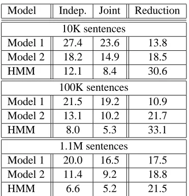
Model Indep. Joint Reduction
10K sentences
Model 1 27.4 23.6 13.8
Model 2 18.2 14.9 18.5
HMM 12.1 8.4 30.6
100K sentences
Model 1 21.5 19.2 10.9
Model 2 13.1 10.2 21.7
HMM 8.0 5.3 33.1
1.1M sentences
Model 1 20.0 16.5 17.5
Model 2 11.4 9.2 18.8
HMM 6.6 5.2 21.5
[image:6.612.93.279.54.247.2]Table 1: Comparison of AER between independent and joint training across different size training sets and different models, evaluated on the development set. The last column shows the relative reduction in AER.
Table 1 shows a summary of the performance of independently and jointly trained models under var-ious training conditions. Quite remarkably, for all training data sizes and all of the models, we see an appreciable reduction in AER, especially on the HMM models. We speculate that since the HMM model provides a richer family of distributions over alignments than either models 1 or 2, we can learn to synchronize the predictions of the two models, whereas models 1 and 2 have a much more limited capacity to synchronize.
Table 2 shows the HMM models compared to model 4 alignments produced by GIZA++ on the test set. Our jointly trained model clearly outperforms not only the standard HMM but also the more com-plex IBM 4 model. For these results, the threshold used for posterior decoding was tuned on the devel-opment set. “GIZA HMM” and “HMM, indep” are the same algorithm but differ in implementation de-tails. The E→F and F→E models benefit a great deal by moving from independent to joint training, and the combined models show a smaller improve-ment.
Our best performing model differs from standard IBM word alignment models in two ways. First and most importantly, we use joint training instead of
Model E→F F→E Combined
GIZA HMM 11.5 11.5 7.0
GIZA Model 4 8.9 9.7 6.9
HMM, indep 11.2 11.5 7.2
HMM, joint 6.1 6.6 4.9
Table 2: Comparison of test set AER between vari-ous models trained on the full 1.1 million sentences.
Model I+V I+P J+V J+P
10K sentences
Model 1 29.4 27.4 22.7 23.6 Model 2 20.1 18.2 16.5 14.9
HMM 15.2 12.1 8.9 8.4
100K sentences
Model 1 22.9 21.5 18.6 19.2 Model 2 15.1 13.1 12.9 10.2
HMM 9.2 8.0 6.0 5.3
1.1M sentences
Model 1 20.0 19.4 16.5 17.3
Model 2 12.7 11.4 11.6 9.2
[image:6.612.323.531.55.133.2]HMM 7.6 6.6 5.7 5.2
Table 3: Contributions of using joint training versus independent training and posterior decoding (with the optimal threshold) instead of Viterbi decoding, evaluated on the development set.
independent training, which gives us a huge boost. The second change, which is more minor and or-thogonal, is using posterior decoding instead of Viterbi decoding, which also helps performance for model 2 and HMM, but not model 1. Table 3 quan-tifies the contribution of each of these two dimen-sions.
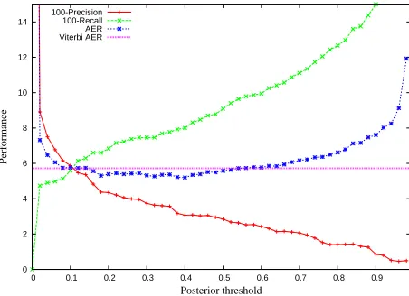
Posterior decoding In our results, we have tuned
our threshold to minimize AER. It turns out that AER is relatively insensitive to the threshold as Fig-ure 2 shows. There is a large range from 0.2 to 0.5 where posterior decoding outperforms Viterbi de-coding.
Initialization and convergence In addition to
[image:6.612.336.516.180.373.2]0 2 4 6 8 10 12 14
0 0.1 0.2 0.3 0.4 0.5 0.6 0.7 0.8 0.9
Performance
Posterior threshold
[image:7.612.75.301.61.225.2]100-Precision 100-Recall AER Viterbi AER
Figure 2: The precision, recall, and AER as the threshold is varied for posterior decoding in a jointly trained pair of HMMs.
HMM model. If we initialize the HMM model with uniform translation parameters, the HMM converges to a completely senseless local optimum with AER above 50%. Initializing the HMM with model 1 pa-rameters alleviates this problem.
On the other hand, if we jointly train two HMMs starting from a uniform initialization, the HMMs converge to a surprisingly good solution. On the full training set, training two HMMs jointly from uni-form initialization yields 5.7% AER, only slightly higher than 5.2% AER using model 1 initialization. We suspect that the agreement term of the objective forces the two HMMs to avoid many local optima that each one would have on its own, since these lo-cal optima correspond to posteriors over alignments that would be very unlikely to agree. We also ob-served that jointly trained HMMs converged very quickly—in 5 iterations—and did not exhibit over-fitting with increased iterations.
Common errors The major source of remaining
errors are recall errors that come from the shortcom-ings of the HMM model. The E→F model gives 0 probability to any many-to-one alignments and the F→E model gives 0 probability to any one-to-many alignments. By enforcing agreement, the two mod-els are effectively restricted to one-to-one (or zero) alignments. Posterior decoding is in principle ca-pable of proposing many-to-many alignments, but these alignments occur infrequently since the poste-riors are generally sharply peaked around the Viterbi
alignment. In some cases, however, we do get one-to-many alignments in both directions.
Another common type of errors are precision er-rors due to the models overly-aggressively prefer-ring alignments that preserve monotonicity. Our HMM model only uses 11 distortion parameters, which means distortions are not sensitive to the lex-ical context of the sentences. For example, in one sentence, le is incorrectly aligned to the as a mono-tonic alignment following another pair of correctly aligned words, and then the monotonicity is broken immediately following le–the. Here, the model is insensitive to the fact that alignments following arti-cles tend to be monotonic, but alignments preceding articles are less so.
Another phenomenon is the insertion of “stepping stone” alignments. Suppose two edges (i, j) and
(i+4, j+4)have a very high probability of being in-cluded in an alignment, but the words between them are not good translations of each other. If the inter-vening English words were null-aligned, we would have to pay a big distortion penalty for jumping 4 positions. On the other hand, if the edge(i+2, j+2)
were included, that penalty would be mitigated. The translation cost for forcing that edge is smaller than the distortion cost.
4.2 BLEU evaluation
To see whether our improvement in AER also im-proves BLEU score, we aligned 100K English-French sentences from the Europarl corpus and tested on 3000 sentences of length 5–15. Using GIZA++ model 4 alignments and Pharaoh (Koehn et al., 2003), we achieved a BLEU score of 0.3035. By using alignments from our jointly trained HMMs instead, we get a BLEU score of 0.3051. While this improvement is very modest, we are currently inves-tigating alternative ways of interfacing with phrase table construction to make a larger impact on trans-lation quality.
5 Related Work
in our work is that we rely exclusively on data like-lihood to guide the two models in an unsupervised manner, rather than relying on an initial handful of labeled examples.
The idea of exploiting agreement between two la-tent variable models is not new; there has been sub-stantial previous work on leveraging the strengths of two complementary models. Klein and Man-ning (2004) combine two complementary mod-els for grammar induction, one that modmod-els con-stituency and one that models dependency, in a man-ner broadly similar to the current work. Aside from investigating a different domain, one novel aspect of this paper is that we present a formal objective and a training algorithm for combining two generic mod-els.
6 Conclusion
We have described an efficient and fully unsuper-vised method of producing state-of-the-art word alignments. By training two simple sequence-based models to agree, we achieve substantial error re-ductions over standard models. Our jointly trained HMM models reduce AER by 29% over test-time intersected GIZA++ model 4 alignments and also increase our robustness to varying initialization reg-imens. While AER is only a weak indicator of final translation quality in many current translation sys-tems, we hope that more accurate alignments can eventually lead to improvements in the end-to-end translation process.
Acknowledgments We thank the anonymous
re-viewers for their comments.
References
Avrim Blum and Tom Mitchell. 1998. Combining Labeled and Unlabeled Data with Co-training. In Proceedings of the
COLT 1998.
Peter F. Brown, Stephen A. Della Pietra, Vincent J. Della Pietra, and Robert L. Mercer. 1994. The Mathematics of Statistical Machine Translation: Parameter Estimation. Computational
Linguistics, 19:263–311.
Michael Collins and Yoram Singer. 1999. Unsupervised Mod-els for Named Entity Classification. In Proceedings of
EMNLP 1999.
Abraham Ittycheriah and Salim Roukos. 2005. A maximum entropy word aligner for arabic-english machine translation. In Proceedings of HLT-EMNLP.
Dan Klein and Christopher D. Manning. 2004. Corpus-Based Induction of Syntactic Structure: Models of Dependency and Constituency. In Proceedings of ACL 2004.
Philipp Koehn, Franz Josef Och, and Daniel Marcu. 2003. Sta-tistical Phrase-Based Translation. In Proceedings of
HLT-NAACL 2003.
E. Matusov, Zens. R., and H. Ney. 2004. Symmetric word alignments for statistical machine translation. In
Proceed-ings of the 20th International Conference on Computational Linguistics, August.
Robert C. Moore. 2004. Improving IBM Word Alignment Model 1. In Proceedings of ACL 2004.
Robert C. Moore. 2005. A discriminative framework for bilin-gual word alignment. In Proceedings of EMNLP.
Hermann Ney and Stephan Vogel. 1996. HMM-Based Word Alignment in Statistical Translation. In COLING.
Franz Josef Och and Hermann Ney. 2003. A Systematic Com-parison of Various Statistical Alignment Models.
Computa-tional Linguistics, 29:19–51.
Ben Taskar, Simon Lacoste-Julien, and Dan Klein. 2005. A Discriminative Matching Approach to Word Alignment. In
Proceedings of EMNLP 2005.
L. G. Valiant. 1979. The complexity of computing the perma-nent. Theoretical Computer Science, 8:189–201.
Appendix: Derivation of agreement EM
To simplify notation, we drop the explicit reference to the parameters θ. Lower bound the objective in Equation 3 by introducing a distributionq(z;x)and
using the concavity oflog:
X
x
logp1(x)p2(x)
X
z
p1(z|x)p2(z|x) (4)
≥ X
x,z
q(z;x) logp1(x)p2(x)p1(z|x)p2(z|x)
q(z;x) (5)
= X
x,z
q(z;x) logp1(z|qx()p2(z|x)
z;x) +
C (6)
= X
x,z
q(z;x) logp1(x,z)p2(x,z) +D, (7)
where C depends only on θ but not q and D de-pends onlyq but notθ. The E-step choosesqgiven a fixedθto maximize the lower bound. Equation 6 is exactly P