A hybrid framework for nonlinear dynamic simulations including full field optical measurements and image decomposition algorithms

A hybrid framework for nonlinear dynamic simulations

including full-field optical measurements and image

decomposition algorithms

LAMPEAS, George and PASIALIS, Vasileios

<http://orcid.org/0000-0002-2346-3505>

Available from Sheffield Hallam University Research Archive (SHURA) at:

http://shura.shu.ac.uk/13923/

This document is the author deposited version. You are advised to consult the

publisher's version if you wish to cite from it.

Published version

LAMPEAS, George and PASIALIS, Vasileios (2013). A hybrid framework for

nonlinear dynamic simulations including full-field optical measurements and image

decomposition algorithms. Journal of Strain Analysis for Engineering Design, 48 (1),

5-15.

Copyright and re-use policy

See

http://shura.shu.ac.uk/information.html

Sheffield Hallam University Research Archive

1

A hybrid framework for non-linear dynamic simulations including full-field

optical measurements and image decomposition algorithms

George Lampeas

1

, Vasilis Pasialis

Laboratory of Technology and Strength of Materials, Mechanical Engineering and Aeronautics

Department, University of Patras, 26500 Rion, Greece

1_{e-mail: [email protected], tel: +302610969498}

1. Introduction

Structural design of innovative components for transport vehicle structures involves extensive

Finite Element (FE) simulations in order to analyze the mechanical response of structural elements under

service loads or loading conditions generated by critical events (e.g. impact). Structural dynamics

methods initially focused on natural frequency analysis and were limited to frequency domain forced

response analysis. Until the mid 70's, transient response analysis was typically performed in the modal

space retaining only the first few fundamental modes of vibration. Dynamic response of non-linear

systems was limited in the frequency-domain and time-domain calculations were rarely attempted due to

numerical instability problems entailed by forward-marching solutions. Generally speaking, time-domain

calculations for non-linear systems, especially in case of impulsive loads, present a severe problem in the

fact that numerical stability is reached as the time-step size is in the range of 1e-8 seconds.

The implicit methods, such as the Newmark's b-method, were developed to achieve stable

integration with larger time steps. Hardware improvements along with algorithm advances made it

2

possible to use explicit time-integration techniques also for high-speed events with rapidly changing

contact impact dynamics. This pushed major commercial aircraft manufacturers towards developing their

in-house structural dynamics code in order to analyze impact events.

Presently, commercial codes including explicit schemes, such as Abaqus, LS-Dyna, Pam-Crash,

and others combined with high performance computing resources, can model impact and crashworthiness

events on the whole structure and provide reasonably good estimations on impact strength. Impact

analysis models are usually quite large and include at least some millions of nodes and elements.

Rather than limiting the model size a priori, one should find algorithms able to simulate the actual

impact event the most accurately as possible. However, these simulations need reliable validation

techniques, especially in cases that anisotropic materials, complex geometry, non-linear dynamic loading

and complex boundary conditions are involved.

In this frame, the use of full-field optical techniques can be proven a useful tool for the deeper

understanding of deformation and failure process of the structural elements, as well as they can be used in

the assessment of the accuracy of numerical results by comparing the predicted values to corresponding

experimental data [1]. The strength of full-field optical techniques is that the entire displacement field can

be visualized and analyzed. By using High Speed cameras, the Digital Image Correlation (DIC) method

can be applied to highly non-linear dynamic events and give quantitative information on the

three-dimensional displacement and strain fields [2].

The Digital Image Correlation method (DIC) has been selected for the present research because,

unlike moire, speckle and holography, it does not require any phase unwrapping and can hence

intrinsically deal with non-smooth displacement / strain distributions. Furthermore, it is relatively fast and

hence highly suited for application in industrial environment.

The objective of the present paper is to integrate full-field optical measurement methodologies

3

order to validate the numerical simulation. The paper focuses on the methodology for comparing

experimental and numerical data. More specifically, the conventional approach of identifying hot-spots in

the data and checking if experiments agree well with simulation results may lead to miss essential details

on the mechanical response of the structure that should be introduced in the simulation models in order to

increase their robustness and predictive capability. Significant progress has been performed in the frame

of project ADVISE [3] in developing an integrated methodology for comparing FE simulations to

experimental data, including the use of reduced or decomposed data (Figure 1) [3]. Different shape

descriptors (Geometric moments, Zernike moments, Chebyshevfeatures, etc.) can be used to significantly

reduce the amount of the data in order to simplify the data comparison [4].

The validity of the proposed methodology is demonstrated for the case of a car bonnet frame

structure of dimensions about 1.8 x 0.8 m, made of PolyPropylene (PP) or PolyAmide (PA) glass fiber

reinforced thermoplastic materials. In purpose of assessing their energy absorption capability, bonnet

frames have been tested in hard-body low velocity, low energy, mass-drop impact loading, in a

drop-tower, with impact energies ranging from 50J to 200J. In parallel, simulation models of the car bonnet

frame have been developed using layered shell elements. A node-to-surface contact definition is

introduced for modeling the physical contact between the impactor and the bonnet.

A High Speed Image Correlation system was used to record full field optical measurement data,

which were used to correlate experimentally recorded and numerically calculated displacement / strain

histories at various points of the structures and different time intervals of the event. In such a way,

numerical simulations of car bonnet frame impact were validated by full field optical measurements.

After decomposition of displacement images captured at time intervals of interest, a reconstruction

process is executed, in order to assess the quality of the decomposition process. Consequently, the

4

2. Low velocity impact tests carried out on the car bonnet.

An Instron 9000 series mass-drop tower capable of delivering up to 1000 J impacting energy was

used. Moreover, the Dantec Dynamics Q-450 high speed optical system was deployed to capture strain /

displacement fields during the dynamic events. The optical system includes two high speed cameras,

mounted on a tripod, capable to capture three-dimensional (3D) fields, an integrated analogue data

acquisition system, a portable notebook and a high intensity white light source. Furthermore, for testing

purposes, a steel base was designed and constructed to provide a robust support for the car bonnet

specimens. The experimental set-up is presented in Figure 2.

The impacting energy, originating from gravitational energy, ranged from 50 to 200J and delivered

through a rigid cylindrical impactor with a hemispherical tip of 25mm diameter. The car bonnet frame

specimens (Figure 3), provided by Centro Ricerche Fiat (CRF), were produced by two material types, i.e.

Polypropylene reinforced with 30% glass fiber (PP) and Polyamide reinforced with 30% glass fiber (PA).

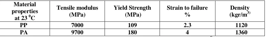
The PA material has greater ductility and higher ultimate strength. The mechanical properties of both

materials are summarized in Table 1.

Specimens were fixed in a horizontal position, in the three hinge areas marked in Figure 3, while

the entire structure was allowed to move only in the upwards out-of-plane direction. Impact took place at

a central point of the bonnet marked with yellow in Figure 3. The acquisition data frequency of the

optical system was set to 4000Hz, resulting in 4 pictures per one millisecond.

Figure 4 shows the images of the damaged specimens taken for the case of PP bonnet (left) and

PA bonnet (right) after impacting with 200J energy. Bonnet made of PA absorbed almost all of the

5

3. FE simulation of the car bonnet impact tests

A stress-check finite element model of the car bonnet frame with an accurate geometry description

has been provided by Centro Ricerche Fiat (CRF) along with bonnet specimens, in the frame of the

ADVISE project [3]. This rough numerical model has been modified, to make it suitable for the

simulation of drop-tower impact events carried out with the ANSYS LS-Dyna FE solver.

The modified FE model comprises 22328 elements. The element type used is ‘Shell 181’, which is

suitable for analyzing thin to moderately-thick shell structures. It is a 4-node element with six degrees of

freedom at each node: translations in the x, y, and z directions, and rotations about the x, y, and z-axes.

There are 5 integration points through-the-thickness. The average thickness of the elements is 3mm. A

finer mesh has been generated in correspondence of the region of impact (Figure 5), because this is the

area facing the impact: consequently, displacement and strain gradients caused by damage propagation

will be much sharper than in the rest of the model.

The finer mesh has been obtained by progressively splitting the elements around the critical impact

zone until convergence of the FE results occurs. The resulting FE mesh includes elements having edge

length equal to about 1/3 of the initial elements. It should be noted that a denser mesh not only facilitates

the convergence of FE analysis but also minimizes errors caused by the condensation techniques applied

later.

Boundary conditions are introduced at nodes of the hinged areas in fashion of displacement

constraints in the coordinate directions x, y and z.

An elastoplastic material model with isotropic damage (MAT2) is used. This model has been

calibrated for the materials used in the case of the simple flat panels simulation [5]. Element failure is

predicted to occur when strain exceeds the corresponding strain to failure limit set to 4% for PA material

and 2.3% for PP material, respectively. The impactor is modelled as a rigid sphere. The node-to-surface

6

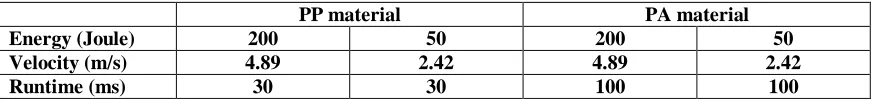
bonnet. An appropriate initial velocity is given to the impactor in order to develop the desired impact

energy values (see Table 2). For example, Figure 6 shows the out-of-plane displacement generated in the

PP200J specimen 12ms after the impact.

Figure 6 shows the out-of-plane displacement generated in the PP200J specimen at 12ms after the

7

4. Approximation of displacement field

Comparison between experimental and numerical data is performed on a selected area of 170mm x

45mm, which is located around the impact region of the bonnet (Figure 7). However, numerical results

and experimental data could not be compared over the entire specimen because of space constraints which

made it not feasible to cover the whole surface of the bonnet (more evidence of this can be gathered from

Figure 2).

A quantitative comparison between experimental and numerical data is made through the use of

Zernike moment parameters, which are used as shape descriptors for the decomposition of displacement –

strain maps.

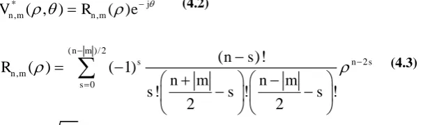
The compared parameter was the out-of-plane displacement field for selected time frames. Eq. 4.1

describes the mathematical expression of the Zernike moment descriptor:

where,

I(ρ,θ)

is the matrix containing displacement/strain data,

*

,

( , )

,

( )

j

n m n m

V

 



R



e



( )/ 2

2 ,

0

(

)!

( )

( 1)

!

!

!

2

2

n m

s n s

n m

s

n

s

R

n

m

n

m

s

s

s







 







 



  







 





 





and

j

 

1

, n is a non-negative integer representing the order of the radial polynomial; m and

n are integers subject to constraints

n



m

even and

m



n

.

2 1 * , , 0 0

1

( , )

( , )

n m n m

n

Z

I

V

d d



 

    







 

(4.1)

(4.2)

[image:8.595.115.424.549.639.2]

8

Since the Zernike polynomials form an orthogonal basis, the original image may easily be

reconstructed as:

, , 0

( , )

_{n m n m}

( , )

n m

I

 

Z

V

 









However, as the reconstruction of an image using infinite number of Zernike moments is not

possible, approximate reconstruction may be achieved by keeping the moments from order 0 to Nmax and

discarding the remaining higher order Zernike polynomials. That is:

max

, , 0

( , )

_{n m n m}

( , )

n m

I

 

Z

V

 









where Nmax is the total number of moments used.

The quality of the reconstruction depends on the number Nmax of Zernike moments used for the

image description. Selection of Nmax can be determined by using a predefined threshold when comparing

the similarity between the original image/map and its counterpart numerically reconstructed.

Two coefficients are usually utilized in literature to assess the accuracy of the Zernike moment

approximation method: the correlation error (Pearson coefficient) and the normalized mean square error,

which can be applied for such comparisons (Eq. 4.6, 4.9). [6, 7]

 

 

 

2

 

₂

ˆ ˆ

ˆ

ˆ ˆ

( , )

I

I

I

I dA

corr I I

I

I

dA

I

I

dA

9

ˆ

ˆ

IdA

,

I

dA

IdA

I

dA

   





∬

∬

∬

∬

The normalized mean square error can be expressed as:

2 2 2

( , )

( , )

( , )

D D

I x y

I x y

dxdy

e

I x y

dxdy

∬

∬

where,

I x y

( , )

and

I x y

( , )

are the original and reconstructed images, respectively.

4.1 Implementation of the shape-descriptors based approximation method

The comparison procedure following the image condensation entails several steps which are

briefly discussed below. First, issues arisen in the post-processing of the numerical and experimental data

were settled appropriately. Due to the non-uniformity of mesh points, a grid of 301x301 points (total

90601 points) was created in the area of interest and both numerical and experimental results are linearly

interpolated on these grid points. The grid density has been defined after a convergence study performed

for the numerical computation of Zernike moments in the unit disc space. Furthermore, the data not

available from experiments because of the presence of fractured and shadowed regions are replaced by

interpolated values suitable for further processing (Figure 8). The same approach is followed for the data

not included in the numerical model because of element elimination after fracture.

It must be stated that the interpolation technique should be applied only in cases when shadowed

areas are relatively small, in order to avoid adding too much arbitrary information into the images.

Furthermore, the interpolation outcome strongly depends on the smoothness of the displacement or strain

(4.9) (4.7)

10

field around the shadowed area. If this field is relatively smooth, as it occurs in the present case, the size

of the surrounding area is not critical. However, if the surrounding field has high gradients, then the result

will depend on the surrounding area size and a parametric study will be necessary to assess the effect of

this size on the interpolation results. Under such scenario, the interpolation method may even be not

applicable and other shape descriptors (e.g. discrete shape descriptors) should be used to condense the

strain field data.

The selection of the total number of Zernike moments is defined such that the normalized mean

error calculated in all cases examined does not exceed 2%. Increasing this threshold results in a higher

image condensation by calculating less shape descriptors with greater loss of image information. Loss of

image information cannot be avoided but should be limited as most as possible. For example, image

mapping to a unit disc entails two steps:

a) Image is decomposed in Nmax Zernike moments, where Nmax is the maximum number of Zernike

moments that can be calculated before numerical instabilities occur. Numerical instabilities can be dealt

using various techniques which allow Zernike moments to be calculated [8, 9]. In this study, 420 Zernike

moments were used for the first step of the condensation process. Figure 9b depicts an example of image

reconstruction with 420 moments. The correspondence existing between the original and the

reconstructed images is quantified by the value of normalized mean error that is equal to 0.36%.

b) Condensation process can be performed more efficiently by computing only the most important

Zernike moments among those computed before. The measure of a moment’s contribution to the image

description is its magnitude, therefore only the greatest moment magnitudes must be considered. In

Figure 9, the original image reconstructed with the 26 most important Zernike moments is displayed. The

computed normalized mean error is equal to 0.78%. Additionally, in Figure 9d the original image

reconstructed with the 52 most important Zernike moments is illustrated, resulting in a slight decrease in

11

moments plot for the PP200J case at 12ms after impact, demonstrating the efficiency of image

condensation with the most important terms.

Defining an optimum mean error to number of moments ratio is currently a matter of interest. In

the present work, the number of moments used for image decomposition was set to 26 moments for all

cases such that no mean error value may exceed the value of 2%.

The displacement field was represented by means of a set of shape descriptors either in the case of FE

results and for the experimentally measured data. While this can be done independently for numerical

simulations and experimental data, the same type and order of shape descriptors should be used, thus

resulting in two feature vectors [10]. Therefore, some extra moments need to be added into DIC map and

the FE map feature vectors so that the moment number of both maps becomes identical and comparison

may correctly be performed. In Table 3 the normalized mean error computed for each case studied and

the number of additional Zernike moments that must be considered are presented. Additionally, the mean

error values are re-calculated taking into consideration these extra moments used.

4.2 Comparison between experimental data and FE results

Once DIC and FE displacement maps vectors were reconstructed, feature vectors obtained for

experimental data and numerical results could be plotted in a FE-moments versus EXP-moments diagram.

By doing this, it was possible to obtain a region where the comparison curve is a straight line inclined by

45° with respect to a horizontal axis [10].

The simpler approach followed in this work adopted histograms. Four cases were compared: three

for PP200J and one for PA50J. Figure 11 presents qualitative comparison between FE and experimental

12

Quantitative comparisons are presented in Figures 12 through Figure 15: the magnitude of

Zernike moments is plotted against the number of moments used in the decomposition. This was done for

both experimental data and FE results. Correlation between experimental data and numerical results is

13

5. Conclusions

In this research, the ‘shape descriptor’ approach was successfully utilized in order to compare

experimental measurements and finite element simulation carried out on a car bonnet frame under highly

non-linear dynamic loading. It can be observed that a low number of terms is required for image

reconstruction of the complex displacement fields of the car bonnet.

Displacement maps gathered from optical methods usually include singular points, right near the

critical areas of the structure (e.g. due to the presence of load introduction devices, strain gages etc.); a

similar scenario occurs in FE simulations when elements are deleted after severe damage propagation, so

that the FE solution can continue without convergence problems. Therefore, the process of selecting an

area for comparisons, converting it to a flat surface and then converting it to rectangular or circular area

without cutouts, which is necessary for the application of shape descriptor approach, requires much effort.

The design of the experimental set up should account for the integration of a full-field optical

system, such that ‘undisturbed’ optical images are obtained and a proper comparison is enabled. The

approach described in [10] is very powerful although complicated. Hence, some automation is required

before routine application.

A very good agreement between experimental measurements and FE results was found in the case

of low-velocity impact tests, taking into account the complexity of geometry and the type of loading

(severe non-linear dynamic). This demonstrates that integration of FE analysis with full-field optical

measurements along with the use of sophisticated comparison techniques can increase design reliability.

In summary, this paper demonstrated that the shape descriptor comparison is a powerful approach

yielding a drastic reduction in computational effort in terms of the quantity of data to be processed. This

makes it possible to carry out reliable comparisons between experimental measurements and simulation

results obtained in the case of large-scale complex structures subject to highly non-linear dynamic

14

6. References

1. Rastogi P, Inaudi D. Trends in optical non-destructive testing and inspection. 1st ed. Amsterdam:

Elsevier, 2000.

2. Siebert Th, Wood R, Splitthof K. High Speed Image Correlation for Vibration Analysis. In: 7th

International Conference on Modern Practice in Stress and Vibration Analysis, Cambridge, UK, 2009.

3. ADVISE – Advanced Dynamic Validations using Integrated Simulation and Experimentation, FP7

project SCP7-GA-2008-218595.

4. Kotoulas L, Andreadis I. Image analysis using moments. In: 5th International Conference on

Technology and Automation, Thessaloniki, Greece, October 2005, pp. 360-364.

5. Lampeas G, Pasialis V, Siebert Th, et al. Validation of impact simulations of a car bonnet by full-field

optical measurements. In: 2nd International Conference on Manufacturing Engineering and Automation,

2011, paper no. AMM.70.57, pp 57-62, Switzerland.

6. Wang W, Mottershead J, Mares C. Mode-shape recognition and finite element model updating using

the Zernike moment descriptor. J Mechanical systems and signal processing 2009; 23: 2088–2112.

7. Liao S, Pawlak M. A Study of Zernike Moment Computing. Lecture Notes in Computer Science.

Computer Vision-ACCV'98, Volume 1351/1997, 394-401, 1997,.

8. Wee C, Paramesran R. On the computational aspects of Zernike moments. J Image and Vision

Computing, 2007; 25: 967–980.

9. Papakostas G, Boutalis Y, et al. Numerical stability of fast computation algorithms of Zernike

15

10. Hack E, Patterson E, Burguete R, et al. A Guideline for the Validation of Computational Solid

Mechanics Models Using Full-Field Optical Data. In: International Conference on Advances in

Experimental Mechanics: Integrating Simulations and Experimentation for Validation, Edinburgh, 2011.

Acknowledgements

The present work has received funding from the European Community Seventh Framework

Programme and specifically under Grant Agreement no. SCP7-GA-2008-218595 ‘Advanced Dynamic

Validations using Integrated Simulation and Experimentation’ (ADVISE).

Figure 1: Validation methodology developed in the frame of ADVISE project.

Figure 2: Experimental set-up, including drop tower, optical system, support base and car bonnet frame

specimen.

Figure 3: Selection of the region of interest where DIC measurements and FE results are compared.

Figure 4: Damage on bonnet of PP material (left) and PA (right) after impact with 200J energy.

Figure 5: View of the convex side of the FE-model of the car bonnet frame with dense mesh on the

impacting area. Gray areas represent the hinged locations.

Figure 6: Numerical out-of-plane displacement field obtained from pp200J bonnet case after 12ms of

impact.

Figure 7: Area selection for comparison.

16

Figure 9: a) Original map taken from the numerical out-of-plane displacement field of pp200J case at 12

ms after impact. b) Original w-displacement map with 420 terms (12 ms after impact). c) Displacement

map with 26 terms, d) Displacement map with 52 terms.

Figure 10: Normalized mean square error versus number of moments plot for the numerical PP200J case

(12ms after impact).

Figure 11: Qualitative comparison between numerical and experimental out-of-plane-displacement fields

for the PP200J case (12 ms after impact).

Figure 12:Comparison between numerical and experimental Zernike moment descriptors for the PP200J

case (4 ms after impact).

Figure 13: Comparison between numerical and experimental Zernike moment descriptors for the PP200J

case (9 ms after impact).

Figure 14: Comparison between numerical and experimental Zernike moment descriptors for the PP200J

case (12 ms after impact).

Figure 15: Comparison between numerical and experimental Zernike moment descriptors for the PA50J

case (3 ms after impact).

List of notations

2

e

Normalized mean square error

17

CRF Centro Ricerche Fiat

I (ρ,θ) Data matrix containing displacement/strain information

I

(ρ,θ) Data matrix containing reconstructed displacement/strain information

PA Polyamide material

PP Polypropylene material

Rn,m Radial polynomial

Vn,m Zernike polynomial

Figure

Figure

Figure

Figure

Figure

Figure

Figure

Figure

Figure

Figure

Figure

Figure

Figure

Figure

Figure

Table 1: Mechanical properties of PP and PA materials at 230 C

Material properties

at 23 0C

Tensile modulus (MPa)

Yield Strength (MPa)

Strain to failure %

Density

(kgr/m3)

PP 7000 109 2.3 1120

PA 9700 180 4 1360

[image:34.612.85.530.100.162.2]

[image:35.612.89.527.91.142.2]

Table 2: Values of parameters used in dynamic FE analyses

PP material PA material

Energy (Joule) 200 50 200 50

Velocity (m/s) 4.89 2.42 4.89 2.42

Runtime (ms) 30 30 100 100

Material type

Impact Energy

(J)

Time after impact

(ms)

Number of additional moments

Normalized mean error %

Numerical

model Experiment

PP 200 4 5 1,07 1,06

PP 200 9 5 0,77 0,71

PP 200 12 2 0,76 0,94

PA 50 3 12 1,88 1,59