Finite element model of a tennis ball impact with a racket
ALLEN, Thomas Bruce
Available from Sheffield Hallam University Research Archive (SHURA) at:
http://shura.shu.ac.uk/3215/
This document is the author deposited version. You are advised to consult the publisher's version if you wish to cite from it.
Published version
ALLEN, Thomas Bruce (2009). Finite element model of a tennis ball impact with a racket. Doctoral, Sheffield Hallam University.
Copyright and re-use policy
teaming and \TServices |
j Collegiate Learning Centre
I
\ Collegiate Crescent UasTipyS | j Sheffield S102BP Iw,.: mu&ak-Mwif.
* Z O
1 0 1 923 0 6 9 X
ProQuest Number: 10701264
All rights reserved
INFORMATION TO ALL USERS
The quality of this reproduction is dependent upon the quality of the copy submitted.
In the unlikely event that the author did not send a com plete manuscript and there are missing pages, these will be noted. Also, if material had to be removed,
a note will indicate the deletion.
uest
ProQuest 10701264
Published by ProQuest LLC(2017). Copyright of the Dissertation is held by the Author.
All rights reserved.
This work is protected against unauthorized copying under Title 17, United States C ode Microform Edition © ProQuest LLC.
ProQuest LLC.
789 East Eisenhower Parkway P.O. Box 1346
Finite Element Model of a Tennis Ball Impact with a Racket
Thomas Bruce Allen
A thesis submitted in partial fulfilment of the requirements of Sheffield Hallam University
for the degree of Doctor of Philosophy
April 2009
Abstract
Previous authors have produced analytical models which accurately simulate tennis impacts. However, currently there are few published studies on the simulation of tennis impacts using finite-element (FE) technique. The purpose of this study was to produce accurate FE models of tennis impacts, which will serve as design tools as well as aid in furthering the understanding of how the ball, string-bed and racket behave during play.
An FE model of a pressurised tennis ball was produced in Ansys/LS-DYNA 10.0 and validated against experimental data. The ball model was updated to simulate the extreme playing temperatures of 10 and 40°C and validated against experimental data, obtained inside a climate chamber. Following validation of the ball model, an FE model of a head-clamped racket was produced and validated against experimental data. The validation included a range of inbound velocities, angles and spin rates, for impacts at a number of nominal locations on the string-bed. Finally, an FE model of a freely suspended racket was constructed and validated against experimental data. Impacts were simulated at a number of nominal impact locations on the string-bed, with a range of ball inbound velocities, angles and spin rates. The impacts were
recorded using two Phantom v4.2 high-speed cameras and analysed in 3D. The
FE models were all in good agreement with the experimental data, for the individual stages of the validation.
A parametric modelling program was produced to be used in conjunction with the model. This program enables the user to adjust a variety of parameters, such as the inbound velocity of the ball, impact location and mass of the racket, and run simulations without any specialist knowledge of the FE model. This program was used to analyse the model against ball to racket impact data obtained during player testing. There was relatively good agreement between the model and player testing data.
Acknowledgements
I would like to thank Dr Simon Goodwill and Professor Steve Haake for their continual support, guidance and enthusiasm throughout the study. This thanks extends to all other members of the Sports Engineering Research Group at Sheffield Hallam University, in particular; Amanda Brothwell and Carole Harris for providing administrative support, Terry Senior for providing technical support, John Kelley for continual assistance and Simon Choppin for assisting with 3D validation techniques and providing player testing data.
I am also grateful to Prince for their sponsorship of the project. The expertise
bought to the project by all of the members of the Prince engineering team, in particular Mauro Pezzato, has been invaluable.
I am thankful to the International Tennis Federation (ITF) for allowing the use of their impressive testing facilities.
Contents
ABSTRACT II
ACKNOWLEDGEMENTS III
CONTENTS IV
LIST OF FIGURES VII
LIST OF TABLES XIX
NOMENCLATURE XXI
1. INTRODUCTION 1
1.1. Motivation for the Research 1
1.2. Aim and objectives 2
1.3. Thesis structure 2
2. LITERATURE REVIEW 4
2.1. Introduction 4
2.2. The ball 5
2.3. The string-bed 14
2.4. The racket 24
2.5. Player testing 34
2.6. Modelling 38
2.7. The influence of technological advances on tennis 49
2.8. Overview of Ansys/LS-DYNA 52
2.9. Discussion 54
2.10. Chapter summary 58
3. TENNIS BALL MODEL 59
3.1. Introduction 59
80 89 89 90 90 91 94 97 111 115 128 129 129 130 136 147 157 158 159 159 159 166 167 167 168 168 168 176 178 180 181 182 182 Validation of the tennis ball model for different temperatures
Chapter summary Practical applications
HEAD-CLAMPED RACKET MODEL
Introduction String properties
Finite element model of a tennis racket string-bed Validation of the string-bed model
Head-clamped racket model
Validation of the head-clamped racket model Chapter summary
FREELY SUSPENDED RACKET MODEL
Introduction
FE Model of a freely suspended tennis racket Validation of the freely suspended racket model
Results and discussion of the freely suspended racket model validation Chapter summary
Practical applications
PARAMETRIC MODELLING PROGRAM
Introduction
Description of the parametric modelling program Discussion
Chapter summary Practical applications
COMPARISON OF THE FE MODEL WITH SIMULATED PLAY
Introduction Method Results
Discussion of player testing Summary of player testing analysis Chapter summary
APPLICATIONS OF THE MODEL
Introduction
8.2. Method 182
8.3. Results 186
8.4. Explanation of results 202
8.5. Chapter summary 222
9. CONCLUSIONS 223
9.1. Introduction 223
9.2. Summary of research 223
9.3. Conclusions 226
9.4. Future research 227
REFERENCES 231
PERSONAL BIBLIOGRAPHY 241
A BALL MODEL VALIDATION 242
A .I. Ball model mesh convergence study 242
A.2. Impact rig validation 244
A.3. Frequency analysis 244
B HEAD-CLAMPED RACKET MODEL 247
B.l. Calculating the impact position on the string-bed 247
B.2. Effect of inbound spin 253
B.3. Difference between string-bed and head-clamped racket model 254
C ALTERNATIVE SPIN CALCULATION 258
List of figures
Figure 2.1 Variation in a) COR and b) contact time, between different balls for
perpendicular impacts on a rigid surface (Haake et al., 2003a)...7
Figure 2.2 Quasistatic material properties of the a) rubber core and b) felt cover of a tennis ball (Goodwill et al., 2005)... 8 Figure 2.3 Ball impact properties for a perpendicular impact on a rigid surface a) Force plot and b) COM displacement and maximum deformation (Goodwill,
2002) 11
Figure 2.4 a) Dynamic string tester and b) Dynamic stiffness and contact
duration results for a selection of strings (Cross et al. 2000)... 18
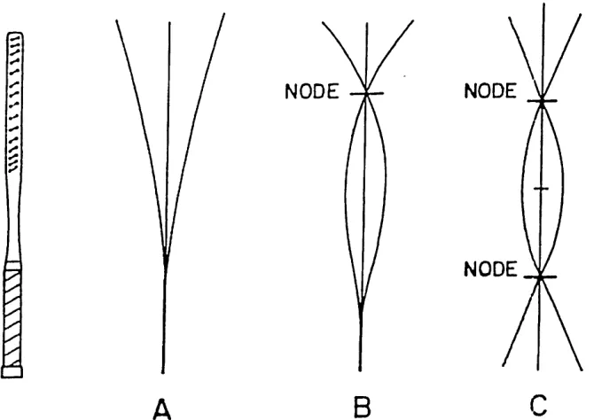
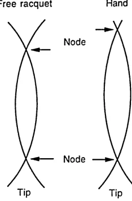
Figure 2.5 Typical material curves which are used for obtaining the dynamic stiffness of different strings (Jenkins, 2003)... 19 Figure 2.6 Analysis of an impact of a ball on a string-bed with an inbound velocity, angle to the racket plane and backspin of 3.27 m s'1, 58.5° and 34.9 rad s'1, respectively (Cross, 2003)...22 Figure 2.7 Horizontal and vertical coefficient of restitution of balls incident at 39° on a head-clamped racket (Goodwill and Haake, 2004a)...23 Figure 2.8 A selection of tennis rackets a) 1981 Dunlop Maxply, b) 1977 Prince oversize and c) 1980 Dunlop Max 200G...25 Figure 2.9 Racket properties from 1870 to 2007 a) frequency and b) mass (Haake et al., 2007)... 26 Figure 2.10 Typical lay-up for a composite tennis racket (Jenkin, 2003)...28 Figure 2.11 Racket frequency response A & B) low frequency handle clamped and c) freely suspended (Brody, 1987)... 29 Figure 2.12 Vibration modes of a free and hand held tennis racket (Cross, 1998)...31 Figure 2.13 Variation of ACOR with impact location for a perpendicular impact between a tennis ball and freely suspended racket (Modified from Brody, 1997a)... 32 Figure 2.14 Shearing of the felt during an oblique impact on a rigid surface at 15
m s'1 and 30° with no initial spin (Goodwill et al., 2005)...41
Figure 4.19 Effect of inbound spin on the experimental data for the head- clamped racket model a) inbound velocity, b) inbound angle and c) impact distance from the long axis of the racket... 118 Figure 4.20 Horizontal and vertical COR for oblique spinning impacts on a head-clamped racket a) centre, b) off-centre, c) tip and d) throat... 120 Figure 4.21 Definition of horizontal COR... 120 Figure 4.22 Rebound topspin for oblique spinning impacts on a head-clamped racket a) centre, b) off-centre, c) tip and d) throat... 121 Figure 4.23 Results for a centre impact on the head-clamped racket model at 21 m-s"1 and 38° with a-c) no spin, d-f) 200 rad-s'1 backspin, g-i) 400 rad-s'1 backspin, j-l) 600 rad-s'1 backspin... 122 Figure 4.24 Impact positions on the string-bed... 123 Figure 4.25 Results obtained from the head-clamped racket model for impacts with an inbound velocity of 20 m-s'1, an angle of 40° and backspin of 200 rad-s'1 at a range of locations on the string-bed a) velocity, b) angle, c) spin... 125 Figure 4.26 Effect of impact position on the deformation of the string-bed of a tennis racket... 126 Figure 5.1 FE model racket geometry with three separate sections... 131 Figure 5.2 Bifilar Suspension used to obtain the polar moment of inertia of a tennis racket... 132 Figure 5.3 The relationship between apparent Young's modulus and natural frequency for the racket in the FE model... 134
Figure 5.4 Convergence of the freely suspended racket model...136 Figure 5.5 a) Impact rig used for simulating impacts on a freely suspended tennis racket (Modified from Choppin, 2008) b) Optimum camera positions for measuring the trajectory of a tennis ball in 3D (Modified from Choppin, 2008). ... 137 Figure 5.6 Impact positions on the string-bed for the validation of the freely suspended racket model for perpendicular impacts... 138 Figure 5.7 Racket positioning for perpendicular and oblique impacts on a freely
suspended racket (View from above)... 139
Figure 6.7 Ball diameter for a 40 m-s'1 perpendicular impact at the GSC of a freely suspended racket a) Ball diameter from ANSYS/LS-Dyna and b) Ball deformation calculated in the results program...166 Figure 7.1 Comparison of the racket in the FE model and the ITF Carbon Fibre racket with each of the 19 players' rackets, a) length, b) width, c) mass and d) balance point...171 Figure 7.2 Comparison of the racket in the FE model and the ITF test racket with a selection of the players' rackets, a) length, b) width, c) mass and d) balance point...173 Figure 7.3 Impact positions a) player testing and b) FE simulations... 174 Figure 7.4 Comparison of rebound velocity from the player testing and FE model a) Horizontal, b) Vertical (perpendicular to string-bed) and c) Resultant (Player data from Choppin etal. (2007a & b))...177 Figure 7.5 Comparison of rebound angle from the player testing and FE model (relative to racket normal) (Choppin et al., 2007a & b)... 178 Figure 7.6 Comparison of rebound topspin from the player testing and FE model (Player data from Choppin etal., 2007a & b)... 178 Figure 8.1 Impact locations on the string-bed used to determine the effect of different racket parameters... 183 Figure 8.2 Relationship between the mass of the racket in the FE model and a) its natural frequency, b) its moment of inertia...184 Figure 8.3 Relationship between the position of the balance point of the racket in the FE model and a) natural frequency, b) moment of inertia... 186 Figure 8.4 Effect of the structural stiffness of a tennis racket on the rebound velocity of the ball, for an impact at 35 m-s'1 and 20° with 300 rad-s'1 of backspin... 187 Figure 8.5 Effect of the structural stiffness of a tennis racket on the longitudinal rebound angle of the ball, for an impact at 35 m-s'1 and 20° with 300 rad-s"1 of backspin...188 Figure 8.6 Effect of the structural stiffness of a tennis racket on the horizontal rebound angle of the ball, for an impact at 35 m-s'1 and 20° with 300 rad-s"1 of backspin...189
Figure 8.7 Effect of the structural stiffness of a tennis racket on the rebound sidespin of the ball, for an impact at 35 m-s'1 and 20° with 300 rad-s'1 of backspin... 190 Figure 8.8 Effect of the structural stiffness of a tennis racket on the rebound topspin of the ball, for an impact at 35 m-s'1 and 20° with 300 rad-s'1 of backspin... 191 Figure 8.9 Diagram to illustrate the difference between using a stiff and flexible racket when performing a forehand shot...192 Figure 8.10 Effect of the mass of a tennis racket on the rebound velocity of the ball, for an impact at 35 m-s'1 and 20° with 300 rad-s'1 of backspin...193 Figure 8.11 Effect of the mass of a tennis racket on the longitudinal rebound angle of the ball, for an impact at 35 m-s'1 and 20° with 300 rad-s'1 of backspin.
...194 Figure 8.12 Effect of the mass of a tennis racket on the horizontal rebound angle of the ball, for an impact at 35 m-s'1 and 20° with 300 rad-s'1 of backspin.
Figure 8.19 Effect of the position of the balance point of a tennis racket on the rebound topspin of the ball, for an impact at 35 m-s'1 and 20° with 300 rad-s"1 of backspin... 202 Figure 8.20 Definition of vertical and horizontal velocity for an impact between a tennis ball and freely suspended racket... 203
Figure 8.21 Effect of racket structural stiffness on the vertical velocity of an impact at the tip at 35 m-s'1 and 20° with 300 rad-s'1 of backspin a) Vertical
force, b) Vertical ball velocity, c) Vertical racket tip displacement and d) Vertical racket COM displacement... 204 Figure 8.22 The vertical deformation of a stiff and flexible freely suspended tennis racket for an impact at the tip... 204
Figure 8.23 Effect of racket structural stiffness on the vertical velocity of an impact at the throat at 35 m-s"1 and 20° with 300 rad-s'1 of backspin a) vertical
force, b) vertical ball velocity, c) racket tip displacement and d) racket COM displacement...205 Figure 8.24 The vertical deformation of a stiff and flexible freely suspended tennis racket for an impact at the throat... 205 Figure 8.25 Effect of racket mass on the vertical velocity of an impact at the tip at 35 m-s'1 and 20° with 300 rad-s'1 of backspin a) vertical force, b) vertical ball velocity, c) racket tip displacement and d) racket COM displacement 206 Figure 8.26 Effect of racket mass on the vertical velocity of an impact at the throat at 35 m-s'1 and 20° with 300 rad-s'1 of backspin a) vertical force, b) vertical ball velocity, c) racket tip displacement and d) racket COM displacement...207 Figure 8.27 Effect of balance point on the vertical velocity of an impact at the tip at 35 m-s'1 and 20° with 300 rad-s'1 of backspin a) vertical force, b) vertical ball velocity, c) racket tip displacement and d) racket COM displacement 208 Figure 8.28 Effect of balance point on the vertical velocity of an impact at the throat at 35 m-s'1 and 20° with 300 rad-s'1 of backspin a) vertical force, b) vertical ball velocity, c) racket tip displacement and d) racket COM displacement...209 Figure 8.29 Spin generation for an impact close the GSC of a freely suspended racket, with an inbound velocity of 28 m-s'1, angle of 23° and zero spin 210
Figure 8.30 Effect of racket stiffness on an impact at the tip at 35 m-s'1 and 20° with 300 rad-s'1 of backspin a) Horizontal force, b) Horizontal ball velocity, c) Topspin, d) Horizontal tip displacement and e) Horizontal COM displacement.
212
Figure 8.31 The horizontal deformation of a stiff and flexible freely suspended tennis racket for an oblique impact at the tip...212 Figure 8.32 Effect of racket stiffness on an impact at the throat at 35 m-s'1 and 20° with 300 rad-s'1 of backspin a) Horizontal force, b) Horizontal ball velocity, c) Topspin, d) Horizontal tip displacement and e) Horizontal COM displacement.
...213 Figure 8.33 The horizontal deformation of a stiff and flexible freely suspended tennis racket for an oblique impact at the throat... 214 Figure 8.34 Effect of racket mass on an impact at the tip at 35 m-s'1 and 20° with 300 rad-s'1 of backspin a) Horizontal force, b) Horizontal ball velocity, c) Topspin, d) Horizontal tip displacement and e) Horizontal COM displacement.
...215 Figure 8.35 Effect of racket mass on an impact at the throat at 35 m-s'1 and 20° with 300 rad-s'1 of backspin a) Horizontal force, b) Horizontal ball velocity, c) Topspin, d) Horizontal tip displacement and e) Horizontal COM displacement.
216 Figure 8.36 Effect of racket balance point on an impact at the tip at 35 m-s'1 and 20° with 300 rad-s'1 of backspin a) Horizontal force, b) Horizontal ball velocity, c) Topspin, d) Horizontal tip displacement and e) Horizontal COM displacement.
...217 Figure 8.37 Effect of racket balance point on an impact at the throat at 35 m-s"1 and 20° with 300 rad-s'1 of backspin a) Horizontal force, b) Horizontal ball velocity, c) Topspin, d) Horizontal tip displacement and e) Horizontal COM displacement...218 Figure 8.38 Diagram showing a centre and off-centre impact on a freely suspended racket... 219 Figure 8.39 Predicted optimised tennis racket design for all round performance
backspin of 300 rad-s'1. The racket has a mass of 0.348 kg, a natural frequency
of 143 Hz and a balance point 0.396 m from the butt...221
Figure 1.1 Number of elements in the ball model against a) maximum displacement of the ball and b) maximum von Mises stress in the ball 244 Figure 1.2 Frequency results for a 5 m-s'1 impact on a force plate...245
Figure 1.3 Frequency results for a 15 m-s'1 impact on a force plate...245
Figure 1.4 Frequency results for a 25 m-s'1 impact on a force plate...246
Figure 1.5 Horizontal and vertical positions of the centre of the string-bed...247
Figure 1.6 Set-up for 60° impacts, showing the location of the release pin and pivot... 248
Figure 1.7 Calculating the horizontal location of the centre of the string-bed, for 60° impacts... 249
Figure 1.8 Calculating the vertical location of the centre of the string-bed, for 60° impacts...249
Figure 1.9 Calculating impact position at 60° inbound angle... 250
Figure 1.10 Calculating impact position at 60° inbound angle... 250
Figure 1.11 Set-up for 20° impacts, showing the location of the release pin and pivot... 251
Figure 1.12 Obtaining the horizontal position of the centre of the string-bed for 20° impacts... 251
Figure 1.13 Obtaining the horizontal position of the centre of the string-bed for 20° impacts... 252
Figure 1.14 Calculating the impact distance from the string-bed along the horizontal axis for the 20° impacts... 252
Figure 1.15 Calculating impact position at 60° inbound angle... 252
Figure 1.16 Effect of inbound spin inbound on a) velocity, b) angle and c) impact location for the centre impacts... 253
Figure 1.17 Rebound a) velocity, b) angle and c) spin. Inbound velocity = 30 m-s'1, inbound angle = 40°...254
Figure 1.18 Horizontal rebound velocity... 255
Figure 1.19 Vertical rebound velocity...256
Figure 1.20 Rebound spin... 256
Figure 1.21 a) Comparison of measured spin rates from each camera using the revolution method and b) comparison of spin between the angle and revolution
method... 258
Figure 1.22 Calculating tension (T) and extended length (L) (Cross et al., 2000). ...259
Figure 1.23 Modified impact rig (Hammer head replaced with bolt)...260
Figure 1.24 Camera set-up... 261
Figure 1.25 Force versus time for the original impact velocity... 263
Figure 1.26 Force plot - String 1 impact 5 higher velocity...265 Figure 1.27 Force plot for an impact with the hammer head replaced by a bolt
List of tables
Table 2.1 Test limits for ITF approved balls (ITF Technical Department, 2009)..6 Table 2.2 Comparison of ball spin rates from different publications (mean ± SD). ...37 Table 3.1 Richimas tracking repeatability for ball and core impacts on a rigid surface, (valuei/ value2) = SD / SD as a percentage of the mean... 71
Table 5.7 Results of a repeatability test for impacts with low medium and high inbound spin, (value) = SD as a percentage of the mean... 145 Table 5.8 Initial conditions used in the FE model to simulate an impact between a tennis ball and freely suspended racket...146 Table 5.9 RMSE between the FE models and experimental data for rebound velocity, for perpendicular impacts on a freely suspended racket... 148 Table 7.1 Pre-impact conditions from the player testing results (+ x offset = towards inbound path of the ball) (+ y offset = towards tip) (Player data from Choppin etal. (2007a & b))...175 Table 8.1 Impact locations on the string-bed used to determine the effect of different racket parameters... 183 Table 8.2 Two sets of FE simulations used to determine the effect of racket structural stiffness...183 Table 8.3 Two sets of FE simulations used to determine the effect of racket mass. The mass moment of inertia, the polar moment of inertia and natural frequency of the racket in the FE model are also displayed...184 Table 8.4 Density and mass of the separate parts of the racket in the two FE models used to determine the effect of racket mass...184 Table 8.5 Two sets of FE simulations used to determine the effect of the balance point of the racket. The mass moment of inertia, the polar moment of inertia and natural frequency of the racket in the FE model are also displayed.
Nomenclature
Abbreviations
ACOR Apparent coefficient of restitution Page 31
COM Centre of mass
COR Coefficient of restitution Page 7
COF Coefficient of friction
DMA Dynamic Modulus Analysis Page 8
FE Finite element
FFT Fast Fourier transform GSC Geometric string-bed centre ITF International Tennis Federation
RDC Racket diagnostic centre Page 20
RMSE Root mean squared error
SD Standard deviation
SPR Surface pace rating Page 13
TDT Tennis Design Tool Page 96
Roman letters
A Cross sectional area [m2]
E Young's Modulus [N-rrf2]
fn Natural frequency [Hz]
G Shear Modulus [N-rrf2]
1 Moment of inertia [kg-nr2]
K Dynamic modulus of strings [N-rrf1]
k Structural stiffness of racket [N-rrf1]
L Length [m]
m Racket mass [kg]
P Pressure [N-nrf2]
T Period of torsional vibration [s]
V Volume [m3]
Greek letters
V Poisson's ratio
0 Inbound angle relative to racket normal /j Coefficient of friction
1. Introduction
The following chapters contain a three year study into the creation and validation of a finite element (FE) model of an impact between a tennis ball and racket.
1.1. Motivation for the Research
Over the years, tennis technology has developed, which has had an enormous impact on the way the game is played. Racket materials have changed from wood to aluminium, to the oversized, more exotic composite ones used today (Haake et al., 2007). These advances have allowed players to hit shots faster and with greater accuracy (Brody, 1997a), effectively increasing the speed of the game (Brody, 1997b). However, this is also believed to have increased the dominance of the server and there is growing apprehension that this is resulting in a reduction in spectator appeal (Kotze et al., 2000). The International Tennis Federation (ITF) is concerned with maintaining public and commercial interest, in order to prevent the demise of the sport through lack of financial support. To successfully regulate a sport, such as tennis, the governing body needs a full understanding of the physical principles and technologies within the game. Thus, the ITF set up a Technical Department in 1997 in order to monitor and direct scientific advances in the sport (ITF Technical Department, 2009).
As a scientific subject area, tennis is well publicised with advances in knowledge and technology coming from within academia and industry. Researchers, scientists and engineers have simulated the various aspects of the game through conventional laboratory investigations, which can be both costly and time consuming. A large number of published studies have been concerned with creating analytical models. Discrepancies between publications have arisen due to errors and assumptions in both experimental and modelling techniques.
increase the physical understanding of other sports and aid in the design of equipment. This project is concerned with constructing an accurate FE model to form the basis of a tennis racket design tool. The intention of this project is to highlight and explain areas of disagreement between previous studies and also to evaluate the suitability of FE technique for modelling tennis ball impacts.
1.2. Aim and objectives
The aim of this thesis is to create an FE model which accurately simulates tennis ball to racket impacts.
The main objectives are as follows;
1. To review existing literature in the field of tennis ball to court and ball to racket impacts.
2. To produce and validate a realistic FE model of a pressurised tennis ball.
3. To produce and validate a realistic FE model of a pressurised tennis ball impacting a freely suspended racket.
4. To produce a parametric modelling program which enables key parameters of a tennis ball to racket model to be easily adjusted and simulations run without the requirement of using an FE interface.
5. To produce a tool that can aid in the design and development of tennis rackets.
6. To use an FE model of a ball to racket impact to further the scientific understanding of tennis.
1.3. Thesis structure
the model. The first stage will be to construct a realistic FE model of a tennis ball impacting on a rigid surface. This ball model will be developed into a ball to racket model which can simulate the full range of tennis shots encountered during play. A parametric modelling program will also be constructed alongside the FE model. This program will enable a wide variety of simulations, encompassing different tennis shots, to be undertaken efficiently. Finally the applications of the model with regard to the design of tennis rackets will be discussed.
2. Literature Review
2.1. Introduction
There is a large amount of literature on the physics of tennis, dating back as far as 1877 (Raleigh, 1877). Previous research has sought to find a greater scientific understanding of the interaction of the ball with both the court and the racket. Work has often been duplicated, which has led to the establishment of certain conclusions. However, there have also been areas of contradiction. The intention of this literature review is to highlight well established conclusions and attempt to explain the reasons for areas of discrepancy and misunderstanding. This project is concerned with the creation and experimental validation of a finite element (FE) model of an impact between a tennis ball and racket. The most logical method of approaching this problem is to separate it into three stages, as detailed below;
1. Model the interaction of the ball with a rigid surface.
2. Model the interaction of the ball with a string-bed.
3. Model the interaction of the ball with a complete racket.
This literature review aims to follow the same course.
The sponsors of this project are Prince, who are concerned with the manufacture of a wide range of different tennis rackets. The intention of this project is to create a tool which can be used to aid the design of their next generation of rackets. It is therefore important to provide them with an overview of how tennis equipment has changed since the origins of the modern game, as well as how these changes have affected play.
This chapter will analyse existing literature on the physics of tennis. The FE model will be built and validated in stages to ensure the highest possible accuracy. Therefore, the literature review contains separate sections on the ball, string-bed and racket. The impacts simulated in the model must be representative of actual play; hence a section on player testing has been included. The final sections are on previous tennis models and the effects of technological advances on the game.
2.2. The ball
2.2.1. The history of the tennis ball
The modern game of tennis or 'lawn tennis' evolved from real tennis in the 1870's, partly due to the invention of the lawn mower. Initially, solid vulcanised rubber balls were used. Improvements quickly followed, including making the ball hollow and pressurising it, as well as stitching a flannel cover around the core to prevent wear (ITF Technical Department, 2009). Originally, the hollow cores were manufactured from a single clover leaf shaped piece of rubber; this procedure was later replaced with the bonding of two compression moulded half shells. The flannel cover was also replaced by specialist cloth, which was bonded to the cores (ITF Technical Department, 2009). Pressureless or unpressurised balls, which had butadiene rubber (synthetic) cores, came into existence in the 1960's (Haines, 1993). However, the pressureless balls failed to gain popularity and were never widely used. In 1972 the International Tennis Federation (ITF) introduced yellow balls to the rules; this was followed by the high altitude ball in 1989. In 2002 the original ball was replaced by a faster type 1 ball, a type 2 ball which was identical to the original and a slower type 3 ball (ITF Technical Department, 2009).
2.2.2. Rules of tennis balls as set by the ITF
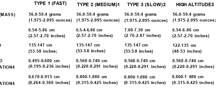
In order to regulate the game of tennis and ensure consistency, any balls used in tournament play must be approved by the ITF. This involves passing a number of assessments, which are mass, size, deformation and rebound. Prior to these assessments, the ball must be acclimatised for 24 hours, at 20 ± 2°C and 60 ± 5% humidity and then compressed. The approval procedures are documented in detail by the ITF (ITF Technical Department, 2009).
balls are summarised in Table 2.1. This study will concentrate on type 2 balls as they are the most commonly used.
Table 2.1 Test limits for ITF approved balls (ITF Technical Department, 2009)
TYPE 1 (FAST) TYPE 2 (MEDIUM)1 TYPE 3 (SLOW)2 HIGH ALTITUDE3 WEIGHT (MASS) 56.0-59.4 grams
(1.975-2.095 ounces) 56.0-59.4 grams(1.975-2.095 ounces) 56.0-59.4 grams(1.975-2.095 ounces)
56.0-59.4 grams (1.975-2.095 ounces;
SIZE 6.54-5.86 cm
(2.57-2.70 inches) 6.5-4-6.86 cm(2.57-2.70 inches) 7.00-7.30 cm(2 76-2.87 inches) 6.54-6.86 cm(2.57-2.70 inches) REBOUND 135-147 cm
(53-58 inches;
135-147 cm
(53-5-8 inches) (53-5-8 inches)135-147 cm (48-53 inches)122-135 cm FORWARD
DEFORMATION4
0.495-0.600 cm
(0.195-0.236 inches) 0.560-0.740 cm(0.220-0.291 inches) 0.560-0.740 cm(0.220-0.291 inches) 0.560-0.740 cm(0.220-0.291 inches) RETURN
DEFORMATION4
0.670-0.915 cm (0.264-0.360 inches)
0.800-1.080 cm
(0.315-0.425 inches) 0.800-1.080 cm(0 315-0.425 inches)
0.800-1 080 cm (0.315-0.425 inches)
2.2.3. The manufacture of tennis balls and their material properties
This study will focus on pressurised tennis balls as they are much more widely used, particularly in tournament play. Detailed descriptions of the current manufacturing process of pressurised tennis balls have been undertaken by both the ITF Technical Department (2009) and Penn (2008). The first stage is to combine natural rubber with additional chemicals and extrude the mixture into pellets. Each of these pellets is compression moulded into a half shell with a wall thickness of approximately 3 mm; pairs of shells are bonded together to form a core. The cores are pressurised to approximately 8.3 * l O ^ N m 2 during the bonding process. The cover consists of two dumb-bell shaped pieces of felt, which are bonded to the core under elevated temperature and pressure using a mould. The white seal is caused by a vulcanised solution, which is applied around the edge of each of the separate pieces of felt before they are bonded to the core.
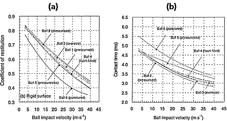
There is very little published data on the material properties of tennis balls. Although, it is predicted that each manufacturer will use slightly different materials and manufacturing procedures, resulting in small variations in impact characteristics (Miller and Messner, 2003). A range of balls can have different dynamic stiffness values even though they have passed the ITF rebound test. This can cause variation in their dynamic properties at high impact velocities
(>10 m-s'1) (Cross, 1999; Haake et ai, 2003a) (Figure 2.1). The ratio of the
(COR). With regard to play, a higher COR would result in an increased speed off the court or racket, whilst dynamic stiffness has been stated to affect the ball's rebound angle (Cross, 1999). Miller and Messner (2003) raised concern that with the current approval procedures, a ball could be introduced with the potential to change the fundamental nature of the game. A possible solution for raising consistency between different balls would be to undertake additional rebound tests at higher impact speeds, as suggested by Cross (1999) and Miller and Messner (2003). Further research would be required to support the introduction of a new standard. A representative ball to surface impact model could be used to accurately predict a ball's rebound characteristics at a range of velocities. Such a model could be used for determining the influence of individual parameters on the game.
n
- - v K - - j • -BaS 2 (pressurised)
JBpII 3 (oversize) 2 0.7
A Dan 1 (pressurised)
. iw . ./ ■ Ba34
(loam Med)
,Ban 5 (pressureless)
(b) Rigid surface ; Bali 6 (punctured) iiUinliiiilnaliDiliu.iliiiiljmi
(b)
5 10 15 20 25 30 35 40 45 Ball impact velocity (m s'1)
Ban 6 (punctured)
Ban 5 (pressureless) * \
/ '
8 4.0 3.5 3.0
, Ban 2
(prfssuris
B3U 3 (oversize)
ll 1 1-1 tlllllllllllllll
» l 1 -1 1 1 1
[image:31.612.99.484.284.489.2]10 15 20 25 30 35 40 45 Ball impact velocity (m s'1)
Figure 2.1 Variation in a) COR and b) contact time, between different balls for perpendicular impacts on a rigid surface (Haake et al., 2003a).
A number of authors have found that the rebound characteristics of tennis balls change with temperature (Rose et al., 2000; Downing, 2007b). The internal pressure of a tennis ball will change with temperature in accordance with the combined gas law (P1V1/T1 = P2V2/T2). It is predicted that this change in internal
temperatures could potentially increase consistency when playing under different atmospheric conditions.
Goodwill et al., (2005) performed materials testing on the rubber core and felt cover, which is used in the construction of a tennis ball. A Hounsfield tensometer was used to obtain the quasi-static stress/strain relationship of the rubber in both tension and compression. The maximum load applied to the rubber samples was 150 N for tension and 450 N for compression (Figure 2.2a). The quasi-static stress/strain relationship of the felt cover was obtained for compression, up to a load of 500 N (Figure 2.2b). Testing the material properties of the rubber and felt from a range of balls would provide an indication of the amount of variation between manufacturers. Testing at a range of temperatures would provide an indication as to how the material properties of tennis balls change with temperature. Dynamic mechanical analysis (DMA) could be used to obtain the viscoelastic properties of the rubber core of a tennis ball (Menard, 2008).
(a) (b)
0.1 0.2 0.3
Strain
-2
3 -—4 ■
1.4
E E
2
M
w
CD 0.6
w 0 .4
-0.2
-0.5 0.1
0 0.2 0.3 0.4
Figure 2.2 Quasistatic material properties of the a) rubber core and b) felt cover of a tennis ball (Goodwill et al., 2005).
Rubber is viscoelastic, which means its properties are both time and temperature dependent. Increasing the strain rate and/or decreasing the temperature results in an increase in the Young's modulus (Menard, 2008). Mase and Kersten (2004) undertook stress relaxation testing on samples taken from the cores of golf balls, in order to obtain their viscoelastic properties. Stress relaxation testing involves measuring the time dependent stress in a
sample held at constant strain, following rapid loading (Menard, 2008). Three point flexure tests were undertaken using a DMA test machine. As the contact time of a golf ball is very small a series of tests were undertaken from -90°C to room temperature. A master curve referenced at room temperature was constructed by undertaking time-temperature superposition on the data obtained from the individual tests. Time-temperature superposition assumes time-temperature equivalence and is used to combine data collected at different temperatures in order to predict the behaviour at a wider frequency range (Menard, 2008). The master curve was fitted to a Prony series and implemented into a model of a golf ball, which was constructed in LS-DYNA. The viscoelastic properties of a tennis ball core could be obtained by undertaking a series of stress relaxation tests across a wide temperature range. However, the contact time of a tennis ball (Goodwill, 2002; Haake et al., 2003a) is approximately 10 times longer than that of a golf ball (Mase and Kersten, 2004). This indicates that the temperature range would not need to be as wide as used by Mase and Kersten (2004).
2.2.4. Tennis ball properties
Downing (2007a) investigated the relationship between static and dynamic tennis ball stiffness. The static stiffness was determined as the amount of forward deformation from an ITF deformation test. The dynamic properties were obtained by projecting balls onto a force plate at velocities in the range from 15 - 30 m-s'1. A higher contact time was stated to indicate a lower dynamic stiffness, as concluded by Dignall and Haake (2000). Downing concluded that there was no relationship between the contact times of tennis balls during dynamic impacts and the amount of forward deformation during a static test. This highlighted that the dynamic properties of tennis balls are more relevant to actual play.
Miller and Messner (2003) measured the COR of tennis balls impacting perpendicular to a rigid surface, for inbound velocities in the range from 7 - 4 5 m-s'1. They concluded that COR decreases with inbound velocity. Although, the decrease in COR, for a set increase in inbound velocity, becomes less pronounced with increasing inbound velocity. COR was stated to decrease from 0.75 at 7 m-s'1, to 0.4 at 45 m-s'1. Miller and Messer also analysed the effect of 'simulated' wear on COR. Wear was simulated by impacting balls obliquely onto a rough block. They concluded that for an inbound velocity of 40 m-s'1, COR decreased significantly at higher numbers of simulated impacts (>100). One hundred impacts were stated to be high, but possibly achievable by a single ball during a match. Measuring additional parameters, such as contact time, deformation and contact force, would have provided a better indication as to how the dynamic properties of a tennis ball change with impact velocity and wear. Other authors have found wear to affect the aerodynamics and hence flight characteristics of tennis balls (Chadwick and Haake, 2000; Goodwill et al., 2004). Further research should be undertaken to determine the typical and maximum amount of wear which a tennis ball will experience when used during match play.
Miller and Messner (2003). Contact time was also found to decrease with inbound velocity, while contact force increased (Figure 2.3a). The peak in contact force at approximately 0.2 ms into the impact has been well reported by numerous authors, and is understood to be due to the walls of the ball buckling
(Cross, 1999; Dignall & Haake, 2000; Goodwill et al., 2005; Haake et al., 2005,
Hubbard & Stronge, 2001; Pratt, 2000). The maximum deformation of the balls was found to increase with inbound velocity (Figure 2.3b). For an inbound velocity of 30 m-s'1 the maximum deformation is approximately equal to the radius of the ball. Goodwill also compared contact times measured with a force plate, with those measured using a high speed video camera. It was difficult to identify the end of contact using the camera, as the balls were still deformed when they left the surface. This led to a discrepancy in the two sets of results and the force plate was stated to be more accurate at measuring contact times.
COM .placement
2 3 4
Time (ms)
o Deformation
e ■ Pressurised » » pressureless o ♦ Oversee o • Punctured
10 20 30
BaB impact velocity (rrVs)
Figure 2.3 Ball impact properties for a perpendicular impact on a rigid surface a) Force plot and b) COM displacement and maximum deformation (Goodwill, 2002).
Rose et al. (2000) analysed the effect of temperature on the properties of tennis
properties of tennis balls cannot be predicted from static tests, in agreement with Downing (2007a).
Downing (2007b) also analysed the effects of temperature, in the range from 10-40°C, on the dynamic properties of tennis balls. COR was found to increase with temperature, in agreement with Rose et al. (2000). Downing also measured contact times, which were found to increase with temperature. This increase in contact time indicates a reduction in the ball's structural stiffness (Dignall and Haake, 2000; Brody et al., 2002; Cross and Lindsey, 2005; Goodwill et al., 2005), which was concluded to be due to a change in the rubber core material properties. The change in the internal pressure of a tennis ball with temperature will also have an effect on its rebound characteristics. Testing punctured balls would remove the effect of the internal pressure. Testing punctured balls and cores would have provided further insight into how the properties of both the rubber and felt change with temperature. However, materials testing would provide the best indication of how the properties of the rubber and felt change with temperature. The change in the internal pressure of a tennis ball with temperature can be calculated if the enclosed volume is assumed to remain constant. Physically measuring the internal pressure at each temperature would be more accurate as it would account for any changes in the diameter of the ball; however, this was neglected by both Rose et al. (2000) and Downing (2007b). Despite using a force plate to measure contact times, Downing did not publish any results for impact forces.
Bridge (1998) examined the effects of changing internal pressure, in the range from 17-98 kPa, on the bounce characteristics of a 'play' ball dropped from a height of 1 m. Contact area and contact time both decreased with increasing internal pressure, whilst COR increased. Bridge concluded that the increase in COR was due to more energy being stored in the compression of the air inside the ball. A similair experiment was undertaken using a squash ball; the change in pressure was replaced with a change in temperature, in the range from 30- 80°C. The contact area, contact time and COR of the squash ball all increased with temperature. Bridge stated that the increase in the flexibility of the rubber with increasing temperature was the dominant factor in determining the rebound characteristics of the ball, rather than the change in internal pressure. This was in agreement with the findings of Downing (2007b) for tennis balls.
During play a tennis ball will impact obliquely to the court surface. When a tennis ball impacts obliquely on a rigid surface the contacting region deforms and flattens, allowing the friction force to reverse if the rotational velocity exceeds the horizontal velocity (Cross, 1999; Haake et al., 2003b). If the reaction force is large enough, the walls of the ball will buckle shortly into the impact, resulting in a cap inverting inside (Dignall & Haake, 2000; Goodwill et al., 2005; Haake eta!., 2005, Hubbard & Strange, 2001; Pratt, 2000), leaving an annulus-contacting region (Cross, 2002). The annulus slides across the surface with a decreasing horizontal speed until the sliding and static friction becomes equal. At this instance the surface tangential velocity of the ball equals its horizontal velocity. This causes the ball to vibrate horizontally, at a frequency determined by its stiffness. In turn, this results in the outer perimeter of the annulus slipping backwards, thus reversing the rotational direction of the ball and creating a higher spin than allowed by the conditions of rolling (Cross,
2002).
Tennis is played on a variety of surfaces, including clay, acrylic and grass. These all affect the balls rebound characteristics in different ways. For example, clay generates high rebound angles, whilst acrylic courts produce lower angles (Haake et al., 2000). The coefficient of friction (COF) is the main factor, which causes the discrepancy in the balls rebound characteristics between individual court surfaces (Brody, 1988).
Downing (2007c) examined the effect of temperature in the range from 10-40°C on surface pace rating (SPR), for an acrylic and synthetic carpet surface. SPR is defined as 100(1- ju), where fj is the COF of the surface. SPR was found to decrease with temperature, indicating an increase in COF. A decrease in SPR equates to the ball losing a higher proportion of its horizontal velocity during the impact. Player testing may also help to provide an insight into how temperature affects the speed of the game on different court surfaces.
order of magnitude stiffer than the ball. FE is a suitable tool that could be used to address this hypothesis, by analysing ball rebound characteristics on surfaces of varying stiffness, corresponding to clay, grass and acrylic.
2.2.5. Summary of the ball
Tennis balls consist of a pressurised rubber core and felt cover. The viscoelastic properties of the rubber core result in a decrease in COR and contact time with increasing inbound velocity. To accurately simulate a tennis ball using FE the viscoelastic properties of the rubber and the internal pressure of the core must be included in the model. The internal pressure and the material properties of the rubber core are dependent on temperature. This means the rebound characteristics of a tennis ball are also dependent on temperature. Therefore, the material properties and the internal pressure used in the model must correspond to the temperature the response of the ball is intended to simulate.
2.3. Th
e string-bed
2.3.1. The history of tennis strings
In the early days of lawn tennis in the 1870's strings were manufactured from sheep intestines or serosa. Sheep intestines were replaced by those of cows, following World War Two (ITF Technical Department, 2009). The relatively high cost of natural gut combined with its poor durability, led to manufacturers using synthetic materials from the 1950's (Haines, 1993). There are now a range of synthetic strings available, including nylon, polyester and Kevlar. The tension at which strings are strung has also changed. In the 1920's the average string tension was 196 N (44 lbs), in comparison to the larger value of 245 N (55 lbs) used today. Professional players have been reported to use string tensions of up to 343 N (77 lbs) (ITF Technical Department, 2009). The width and length of racket heads has also increased considerably since the 1870's, resulting in larger string-beds (Haake et al., 2007). For the same string tension a larger string-bed will have a lower structural stiffness. Therefore, players may have increased the tension of their strings in order to counteract the effects of the larger string-bed.
2.3.2. Rules
The first rule to be introduced by the ITF concerning the string-bed and arguable the most important, was in 1978 and is stated below;
"The hitting surface of the racket shall be flat and consist of a pattern of crossed strings connected to a frame and alternately interlaced or bonded where they cross." (ITF Technical Department, 2009)
This rule was introduced following a novel invention labelled the ‘spaghetti strings’ or ‘spaghetti racket’, where the strings were not interlaced. The 'spaghetti racket1 allowed a player to produce very high spin rates due to large horizontal displacements of the strings during oblique impacts (Goodwill and Haake, 2002).
2.3.3. The manufacture of tennis strings and their material properties
When manufacturing natural gut strings, the first stage is to remove any contaminants from the intestines. This is done using a chemical bath. The strands are then spun, dried and polished to produce a string with the required diameter. The final stage is to apply a protective polyurethane coating (ITF Technical Department, 2009). Synthetic strings are usually constructed by winding hundreds of filaments around a central core (Haines, 1993; ITF Technical Department, 2009). The filaments are constructed with an extrusion mould. The core can either be extrusion moulded as a solid section or constructed by winding together a number of larger diameter filaments. It is widely accepted that the mechanical properties of tennis strings will be determined by the process used to construct them and the choice of materials (Haines, 1993; ITF Technical Department, 2009).
Although the results obtained are useful for comparing different strings, it is predicted that an impact between a tennis ball and racket will result in higher strain rates than those tested by Cross (2000a). Assuming an initial length of 0.3 m, a contact time of 5 ms (Brody et al., 2002; Cross & Lindsey, 2005) and the perpendicular displacement of the string-bed in the range from 0.015 to 0.030 m (Goodwill, 2002), the time-averaged strain rate will be 0.6-2.4 m-s"1. This is in agreement with the approximate strain rate of 40 000 mm/min (0.67 m-s"1) stated by Cross et al. (2000).
Calder et al., (1987) analysed both the static and dynamic properties of a range of tennis strings. A mid-sized tennis racket was strung at 220 N (50 lbs), with a load cell fitted in-line with a central main string. No information regarding the string type or gauge was provided. When the racket was head-clamped and subjected to an impact with a tennis ball, the string tension increased by 90 N and the contact time was approximately 3.5 ms. The inbound velocity of the ball was not stated, and there was no mention as to how this may influence the results. The static properties of the strings were obtained using an Instron machine, with the crosshead speed set to 20 mm/min. A rig was constructed for the dynamic tests, which was capable of applying a load of 90 N to a tensioned string, over a period of 3.5 ms. A large amount of hysteresis was observed, for both the static and dynamic tests, when the strings were loaded to 90 N without any preload. Hysteresis is observed as a difference between a loading and unloading stress-strain curve and is due to the sample softening as a result of stretching (Mullins, 1969). The hysteresis decreased to a negligible amount when the pre-load was increased to 270 N. The stiffness of the synthetic strings increased with both the strain rate and the amount of preload, while the stiffness of the natural gut strings remained virtually constant. The stiffness of all the strings was found to be linearly elastic, under the conditions which Calder et al. obtained from impacting a ball onto a head-clamped racket. Synthetic strings were concluded to be stiffer than natural gut strings under these conditions. The effect of adjusting the applied load was not analysed.
Cross et al. (2000) used a bespoke impact rig to determine the dynamic properties of tennis strings (Figure 2.4a). They stated that a typical impact between a ball and string-bed will have a maximum force of approximately 1500 N and a contact time of around 5 ms. Assuming this load is evenly distributed
(b)
Loulcrl
n**)- • — 300 mm —♦Si ring J m Rod Rod
Tern toning mil Pivot
Wood
250
90 strings
200 CO
Z
U-Kevlar
150
100
204
100 k (kN/m)
150
28 ~ 3
w
Siring lawrfcoim
Figure 2.4 a) Dynamic string tester and b) Dynamic stiffness and contact duration results for a selection of strings (Cross et al. 2000).
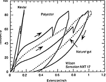
Cross (2001a) derived a method for obtaining the dynamic stiffness of tennis strings within their operational range, using an Instron machine. The first stage is to load a string with a gauge length of 20 mm to 280 N (63 lbs), at a rate of 50 mm/min (0.00083 m-s-1) and hold it for 100s. This is intended to replicate stringing a racket. Following this the string is loaded to 380 N (85.5 lbs) and held for a further 10 s. This is intended to replicate 2000 impacts between a ball and string-bed, each with a contact time of 5 ms. The final stage is to unload the string at a rate of 100 mm/min (0.0017 m-s‘1). The unloading step is stated to produce a curve without any significant creep effects. This is claimed to be the reason why it is possible to obtain dynamic string properties using an Instron machine. Figure 2.5 shows the load extension curves obtained for a range of different strings. The dynamic stiffness is calculated from the unloading curve by dividing the change in load between 311 and 222 N (70 and 50 lbs) with the change in length. The range of 311 - 222 N is used to obtain the dynamic stiffness as this is stated to be the typical operational range of the strings. However, Cross loaded the strings to 380 N to replicate an impact between a ball and string-bed; this indicates inconsistencies in the method.
100
Kevtar
Natural gut V/Json Sensation N X T 17
0.8 1.2
0.6 1
0.4
[image:43.613.199.383.16.157.2]0 0.2
Figure 2.5 Typical material curves which are used for obtaining the dynamic stiffness o f different strings (Jenkins, 2003).
The other property besides structural stiffness, which is believed to distinguish individual tennis strings, is friction. There are currently no published studies on string to string friction. Cross et al. (2000) measured the COF between tennis strings and the felt used to cover the ball. He glued tennis ball felt onto a pipe with a diameter of 60 mm, wrapped a i m length of string around twice and attached a 0.15 kg mass to the end. The force required to lift the mass at a constant velocity, which was not declared, was recorded with a spring balance. The COF for most of the strings was 0.15-0.18, while the lowest and highest obtained values were 0.11 and 0.36, respectively. Cross (2000b) analysed the COF of friction between a ball and string-bed. He experimentally obtained sliding and rolling COF's for five different strings, which were 0.27 - 0.42 and 0.05, respectively. However, he calculated sliding friction by placing masses up to 10 kg on a ball and dragging it across the string-bed, a method not representative of a typical high momentum collision. It is predicted that the ball will deform around the strings due to the applied load; meaning that Cross was actually measuring a traction force rather than a friction force. The relationship between the applied load and coefficient of friction was not investigated. The deformation of the ball around the strings may explain the discrepancy between the COF values obtained by Cross et al. (2000).
2.3.4. Ball to string-bed impacts
majority of the energy is assumed to be stored in the deformation of the ball; when a ball collides with a string-bed the energy is equally divided between both objects (Cross & Lindsey, 2005). During a collision between a ball and a string-bed, the ball loses around 45% of its energy and the string-bed loses around 5% of its energy (Brody et al., 2002; Cross & Lindsey, 2005). Therefore, the ball to string-bed collision is more efficient than a rigid surface impact (Jenkins, 2003; Brody et al., 2002; Cross & Lindsey, 2005). Although there are no set rules, the COR for a tennis ball dropped onto a head-clamped racket from a height of 2.54 m is about 0.75 - 0.8, compared to around 0.74 for a rigid surface (Brody et al., 2002). Reducing string-bed stiffness has the effect of increasing both the rebound velocity of the ball and the contact time, which is approximately 5 ms (Brody et al., 2002; Cross & Lindsey, 2005). The two main factors that determine string-bed stiffness are the string material and tension. The Babolat Racquet Diagnostic Center (RDC) is commonly used as a tool for measuring the quasi-static stiffness of a string-bed (Babolat, 2009). The RDC displaces the centre of the string-bed using a small disk and provides a stiffness value between 0 and 100 in RDC units. The higher the RDC value the stiffer the string-bed.
Stiffness is considered to be the principal factor that separates the different string materials. Polyester strings have high stiffness, causing them to lose tension at an accelerated rate, unlike highly elastic strings, such as natural gut. Tension increases more during impact with polyester strings, resulting in shorter contact times and a "controlled feel". Natural gut on the other hand, produces a more comfortable feel, due to longer contact times (Cross et al., 2000). FE could be use to analyse the variation in contact times and reaction forces for different string types.
String tension, which typically ranges from 220 - 310 N (Brody et al., 2002), affects both rebound velocity (Haake et al., 2003a; Goodwill and Haake, 2004a; Cross & Lindsey, 2005; Brody et al., 2002) and angle (Goodwill and Haake, 2004a & b). However, decreasing tension by 44 N only results in approximately a 2% rise in the rebound velocity of the ball for a ground stroke (Jenkins, 2003; Brody et al., 2002; Cross & Lindsey, 2005). Obtaining an exact string tension may seem irrelevant, particularly when building an FE model which will have an
inevitable margin of error, but it will have a large effect on the ball's rebound angle for oblique impacts.
Grip 30
20
0.5 — 10
LL
-0.5
-10
-20
•2 0 2 4 6 8 10
t (ms)
Figure 2.6 Analysis o f an impact of a ball on a string-bed with an inbound velocity, angle to the racket plane and backspin of 3.27 m-s'1, 58.5° and 34.9 rad-s'1, respectively (Cross, 2003).
Goodwill and Haake (2004a) experimentally analysed the impact of an oblique spinning tennis ball on a head-clamped racket. They tested inbound velocities of 23 and 31 m-s'1 at an angle of 39° to the normal, with backspin in the range from 0-420 rad-s'1. These conditions were stated to be representative of a topspin forehand. The balls had backspin prior to impact due to a change in the Newtonian frame of reference from the court to the racket. A head-clamped racket was used to isolate the string-bed and eliminate the effect of racket parameters, such as stiffness and mass. A range of natural gut and synthetic strings, were tested. Each string was tested at a tension of 40 and 70 lbs (178 and 311 N). The racket type, which remained constant across all the tests, had a head size of 632 cm2. The balls were fired using a modified BOLA (BOLA, 2009) and the impacts were stated to be at the centre of the string-bed. However, there was no evidence to suggest that the impact positions were actually calculated. The impacts were recorded with a high-speed video camera and manually analysed using the bespoke software Richimas V3. The standard deviation in inbound velocity and angle for all the impacts was 0.4 m-s'1 and 0.7°, respectively. The standard deviation obtained from a manual tracking repeatability study was 0.2 m-s'1 for velocity, 0.3° for angle and 25 rad-s'1 for spin. The results showed that the rebound velocity, angle and spin of the ball, all decreased with increasing inbound backspin. The vertical rebound velocity of the ball was virtually independent of inbound backspin (Figure 2.7). The horizontal rebound velocity decreased significantly with inbound backspin
(Figure 2.7). This decrease in horizontal velocity is the main cause of the decrease in the resultant rebound velocity and angle with increasing inbound backspin. Rebound velocity was generally higher for the impacts on the rackets strung at the lower tension of 40 lbs (178 N), in agreement with other authors (Jenkins, 2003; Brody et al., 2002; Cross & Lindsey, 2005). The results indicated that string-bed stiffness does not have an effect on rebound spin. This was in contradiction to the belief of many players. However, there was a large amount of scatter in the experimental data making it difficult to justify a solid conclusion. The horizontal rebound velocity remained effectively constant for the two string tensions, while vertical rebound velocity increased with string tension (Figure 2.7). The rebound angle of the balls (relative to the string-bed normal) was also smaller for the rackets strung at lower tension, in agreement with Goodwill and Haake (2004b). The stiffness of the string-bed had different effects on the horizontal and vertical rebound velocity of the ball. Testing at a range of different inbound angles would provide further insight into the effect of string-bed stiffness on the rebound characteristics of the ball.
Vy(f)/Vy(i)
— 40 lbs 70 lbs 0.4
--500 -400 -300 -200 -100 0 Inbound spin (rad/s)
Figure 2.7 Horizontal and vertical coefficient of restitution of balls incident at 39° on a head-clamped racket (Goodwill and Haake, 2004a).
This is predicted to be due to the difficulty in accurately measuring and adjusting COF.
2.3.5. Summary of the string-bed
The structural stiffness of a tennis racket string-bed, which is determined by the string material and tension, affects the rebound velocity and angle of the ball. Therefore, a method for simulating a tensioned string-bed in an FE model must be developed. The string-bed must consist of interwoven strings with the correct material properties. As tennis strings are viscoelastic dynamic materials testing must be undertaken. However, previous research indicates that tennis strings have linear material properties within their operational range.
2.4. Th
e racket
2.4.1. The history of the tennis racket
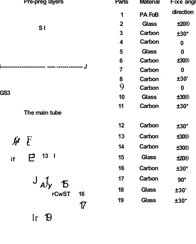
was introduced in 1980 and remained in production for 10 years. The Max 200G was manufactured by injection moulding nylon with short carbon fibres (Haines
et al., 1983). Despite its many production advantages, the manufacturers were unable to use the injection moulding process to produce rackets with the same mass and head size as those produced using composite lay-ups. Currently, the majority of rackets are manufactured from composite lay-ups as this allows materials to be precisely placed for optimum stiffness and weight distribution. Modern composite rackets are around 30% lighter and three times stiffer than their state of the art wooden counterparts. A lighter racket can be swung faster, whilst stiffness increases impact efficiency; both of these factors allow the
player to increase the rebound velocity of the ball (Haake et al., 2007). The
head size of these modern composite rackets is also around 40% larger, which increases ease of play.
Figure 2.8 A selection of tennis rackets a) 1981 Dunlop Maxply, b) 1977 Prince oversize and c) 1980 Dunlop Max 200G.
Haake et al. (2007) measured various properties of 150 tennis racket from the
500
200
420 -160
o o
3
S’ 80 260
Li
-40 18