Continuum Gating Current Models Computed with Consistent Interactions

Article

Continuum Gating Current Models Computed

with Consistent Interactions

Tzyy-Leng Horng,1Robert S. Eisenberg,2,3Chun Liu,2and Francisco Bezanilla4,5,*

1_{Department of Applied Mathematics, Feng Chia University, Taichung, Taiwan;}2_{Department of Applied Mathematics, Illinois Institute of}

Technology, Chicago, Illinois;3Department of Physiology and Biophysics, Rush University, Chicago, Illinois;4Department of Biochemistry and Molecular Biology and Institute for Biophysical Dynamics, University of Chicago, Chicago, Illinois; and5_{Centro Interdisciplinario de}

Neurociencia de Valparaı´so, Facultad de Ciencias, Universidad de Valparaı´so, Valparaı´so, Chile

ABSTRACT The action potential of nerve and muscle is produced by voltage-sensitive channels that include a specialized device to sense voltage. The voltage sensor depends on the movement of charges in the changing electric field as sug-gested by Hodgkin and Huxley. Gating currents of the voltage sensor are now known to depend on the movements of posi-tively charged arginines through the hydrophobic plug of a voltage sensor domain. Transient movements of these permanently charged arginines, caused by the change of transmembrane potential V, further drag the S4 segment and induce opening/closing of the ion conduction pore by moving the S4-S5 linker. This moving permanent charge induces capacitive current flow everywhere. Everything interacts with everything else in the voltage sensor and protein, and so it must also happen in its mathematical model. A Poisson-Nernst-Planck (PNP)-steric model of arginines and a mechanical model for the S4 segment are combined using energy variational methods in which all densities and movements of charge satisfy conservation laws, which are expressed as partial differential equations in space and time. The model computes gating current flowing in the baths produced by arginines moving in the voltage sensor. The model also captures the capac-itive pile up of ions in the vestibules that link the bulk solution to the hydrophobic plug. Our model reproduces the signature properties of gating current: 1) equality of ON and OFF charge Q in integrals of gating current, 2) saturating voltage depen-dence in the Q(charge)-voltage curve, and 3) many (but not all) details of the shape of gating current as a function of voltage. Our results agree qualitatively with experiments and can be improved by adding more details of the structure and its correlated movements. The proposed continuum model is a promising tool to explore the dynamics and mechanism of the voltage sensor.

INTRODUCTION

Much of biology depends on the voltage across cell mem-branes. The voltage across the membrane must be sensed before it can be used by proteins. Permanent charges move in the strong electric fields within membranes, so car-riers of sensing charge were proposed as voltage sensors even before membrane proteins were known to span lipid membranes (1). The movement of permanent charges of the voltage sensor is gating current, and the movement is the voltage-sensing mechanism. Permanent charge is our name for a charge or charge density independent of the local electric field (for example, the charge and charge dis-tribution of Naþbut not the charge in a highly polarizable anion like Br or the nonuniform charge distribution of

H2O in the liquid state with its complex time dependent

(and perhaps nonlinear) polarization response to the local electric field).

Knowledge of membrane protein structure has allowed us to identify and look at the atoms that make up the voltage sensor. Protein structures do not include the membrane potentials and macroscopic concentrations that power gating currents, and therefore, simulations are needed. Atomic-level simulations like molecular dynamics (MD) do not provide an easy extension from the atomic timescale1015s to the bio-logical timescale of gating currents that starts at106 s and reaches102s. Calculations of gating currents from simulations must average the trajectories (lasting101s sampled every 1015s) of106atoms, all of which interact through the electric field to conserve charge and current while conserving mass. It is difficult to enforce continuity of current flow in simulations of atomic dynamics because simulations compute only local behavior, whereas continuity Submitted October 11, 2018, and accepted for publication November 28,

2018.

*Correspondence:[email protected] Editor: Michael Grabe.

270 Biophysical Journal116, 270–282, January 22, 2019 https://doi.org/10.1016/j.bpj.2018.11.3140

2018 Biophysical Society.

of current is global, involving current flow far from the atoms that control the local behavior. It is impossible to enforce con-tinuity of current flow in calculations that assume equilib-rium (zero net flow) under all conditions.

A hybrid approach is needed, starting with the essential knowledge of structure but computing only those parts of the structure used by biology to sense voltage. In close-packed (‘‘condensed’’) systems like the voltage sensor or ionic solutions, ‘‘everything interacts with everything else’’ because electric fields are long ranged as well as exceedingly strong (2). In ionic solutions, ion channels, even enzyme active sites, steric interactions that prevent the overfilling of space in well-defined protein structures are also of great importance because they produce short-range correlations (3).

Closely packed charged systems are well handled math-ematically by energy variational methods. Energy varia-tional methods guarantee that all variables satisfy all equations (and boundary conditions) at all times and under all conditions and are thus always consistent. We use the energy variational approach developed in (4) and (5) to derive a consistent model of gating charge movement, based on the basic features of the structure of crystallized voltage-sensitive channels. A schematic of the model is shown below. The continuum model we use simulates the mechanical dynamics in a single voltage sensor, although the experimental data is from many independent voltage sensors. Ensemble averages of recordings of individual in-dependent voltage sensors are equivalent to macroscopic continuum modeling in a single voltage sensor if correla-tions are captured correctly in the model of the single voltage sensor.

MATERIALS AND METHODS

Theory: Mathematical model

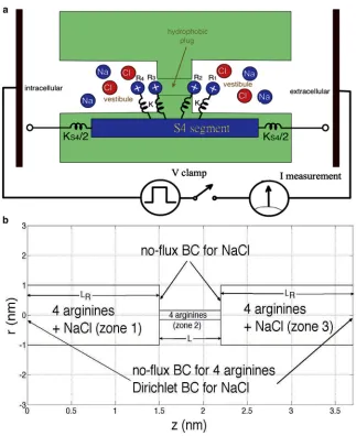
The reduced mechanical model for a voltage sensor is shown inFig. 1a

with four arginines (Ri,i¼1, 2, 3, 4), each attached to the S4 helix by iden-tical springs with the same spring constantK. The electric field will drag these four arginines because each arginine carriesþ1 charge. The charged arginines can also move as a group. S4 connects to S3 and S5 at its two ends by identical springs with spring constantKS4/2.

Once the membrane is depolarized from, for example,90 mV inside negative to þ10 mV inside positive, arginines together with S4 will be driven toward the extracellular side. A repolarization fromþ10 to

90 mV moves the arginines back to the intracellular side. This movement is the basic voltage-sensing mechanism. The movement of S4 triggers the opening or closing of the lower gate—consisting mainly of S6 forming the ion permeation channel—by a mechanism widely assumed to be me-chanical, although electrical aspects of the linker motion are likely to be involved as well.

When arginines are driven by an electric field, they are forced to move through a hydrophobic plug composed of several nonpolar amino acids from S1, S2, to S3 (6). Arginines reside initially in the hydrated lumen of the intracellular vestibule. They then move though the hydrophobic plug and wind up in the vestibule on the extracellular side. This movement in-volves dehydration when the arginines move through the hydrophobic plug, in which the arginines encounter a barrier in the potential of mean

force (PMF), mainly dominated by the difference of the solvation energy in bulk situation and in the hydrophobic plug (7). Note that Naþand Cl (which are the only ions in the bulk solution in this article for simplicity) are found only in vestibules and are not allowed into the hydrophobic plug in our model. The ends of the two vestibules on each side of the hy-drophobic plug act as impermeable walls for Naþand Clin our model. When the voltage is turned on and off, these two walls store/release charge (carried by ions) in their electric double layers (EDL) that have many of the properties of capacitors.

In this continuum model, the four arginines (Ri,i ¼1, 2, 3, 4) are described by their individual density distributions (concentrations) (ci,

i¼1, 2, 3, 4), allowing the arginines to interact with Naþand Clin vestibules. The density (i.e., concentration) distributions represent prob-ability density functions as shown explicitly in the theory of stochastic processes used to derive such equations in (8) using the general methods of (9). The important issue here is how well the correlations are captured in the continuum model. Some are more likely to be faithfully captured in molecular or coarse-grained dynamics simulations (e.g., more or less local hard sphere interactions) (10–14) and others in continuum models (e.g., correlations induced by far-field boundary conditions like the potentials imposed by bath electrodes to maintain a voltage clamp) (15–18).

Here, we treat the S4 itself as a rigid body, so we can capture the basic mechanism of a voltage sensor without considering the full details of struc-ture, which might lead to a three-dimensional model difficult to compute in reasonable time. We construct an axisymmetric one-dimensional (1D) model with a three-zone geometric configuration illustrated inFig. 1b, followingFig. 1a. Zone 1 withz˛[0,LR] is the intracellular vestibule; zone 2 withz˛[LR,LRþL] is the hydrophobic plug; zone 3 withz˛ [LRþL, 2LRþL] is the extracellular vestibule. Arginines, Naþ, and Cl can all reside in zone 1 and 3. Zone 2 only allows the residence of arginines, albeit with a severe hydrophobic penalty because of their permanent charge, in a region of low dielectric coefficient, hence called hydrophobic.

Based onFig. 1 b, the governing 1D dimensionless Poisson-Nernst-Planck (PNP)-steric equations are expressed below with the detailed nondi-mensionalization process shown in Supporting Materials and Methods, Section S1. The first one is a Poisson equation that shows how charge cre-ates potential: 1 A d dz

GAdf dz

¼ X

N

i¼1

qici; i ¼ Na;Cl;1;2;3;4; (1)

wherefis electric potential;ciis concentration of speciesiwith valence

qNa ¼ 1, qCl ¼ 1, qi¼ qarg ¼ 1, i ¼ 1, 2, 3, 4;G¼l2D=R2 with

lD¼

ffiffiffiffiffiffiffiffiffiffiffiffiffiffiffiffiffiffiffiffiffiffiffiffiffiffi εrε0kBT=c0e2

p

being the Debye length, and the characteristic length (radius of vestibule)R¼1 nm here.A(z) is the channel cross-sectional area at positionz. For zones 1 and 3,G¼1 by setting NaCl bulk concentration

c0¼184 mM andεr¼80. For zone 2, we assume a hydrophobic environ-ment withεr¼8 and thereforeG¼0.1. The value of the dielectric constant inside the hydrophobic plug (zone 2) is not experimentally available; how-ever, the computational result is not sensitive to this value based on our sensitivity analysis.

The second equation is the species transport equation based on conserva-tion laws:

vci vt þ

1 A

v

vzðAJiÞ ¼ 0; i ¼ Na;Cl;1;2;3;4; (2)

with the content of fluxJiexpressed below based on the Nernst-Planck equation for Naþand Cl:

Ji ¼ Di vci

vzþciqi

vf vz

; i ¼ Na;Cl; zin zone1and3;

(3)

Gating Currents Model

and for four argininesci,i¼1, 2, 3 and 4 based on the Nernst-Planck equa-tion with steric effect and some imposed potentials:

Ji ¼ Di vCi

vz þqargci

vf vzþci

vVi vz þ

vVb vz

þgci

X

jsi vcj

vz

!

; zin all zones;

(4)

whereDiis the diffusion coefficient for speciesi.

The first and second terms inEqs. 3and4describe diffusion and electro-migration, respectively. The third terms inEq. 4are external potential terms withVi,i¼1, 2, 3, and 4 being the constraint potential for the four arginines

cito S4, represented here by a spring connecting each argininecito S4, as shown inFig. 1a. Governing equationsEqs. 1,2,3, and4were derived by energy variational methods, which is further shown inSupporting Materials and Methods, Section S3.

The elastic system is described by

Viðz;tÞ ¼ Kðz ðziþZS4ðtÞÞÞ2; (5)

whereKis the spring constant,ziis the fixed anchoring position of the spring for each argininecion S4, andZS4(t) is the center-of-masszposition

of S4 by treating S4 as a rigid body. Here, we setz1¼0.6,z2¼0.2,

z3¼ 0.2, andz4¼ 0.6 using structural information that gives the

argi-nine anchoring interval on S4 as 0.4 nm.ZS4(t) follows the motion of

equa-tion based on the spring-mass system:

mS4 d2ZS4

dt2 þbS4 dZS4

dt þKS4ðZS4ZS4;0Þ

¼ X4

i¼1

Kðzi;CM ðziþZS4ÞÞ; (6)

wheremS4,bS4, andKS4are the mass, damping coefficient, and restraining

spring constants for S4.ZS4,0is the resting position ofZS4(t). Here,zi,CMis the center of mass for the set of argininesci, which can be calculated by

zi;CM ¼

RLþ2LR

0 AðzÞzcidz

RLþ2LR

0 AðzÞcidz

;i ¼ 1; 2; 3; 4: (7)

We assume that the spring-mass system for S4 is overdamped, which means the inertia term inEq. 6can be neglected.

The energy barrierVbinEq. 4is nonzero only in zone 2, which mainly represents the difference in solvation energy, chiefly characterized by the FIGURE 1 (a) Geometric configuration of gating pore in this model, including the attach-ments of arginines to the S4 segment. (b) Following (a), an axisymmetric three-zone domain shape is designated in r-zcoordinate for the current 1D model. Here, the diameter of the hydrophobic plug is 0.3 nm (arginine’s diameter);L¼0.7 nm;

LR¼1.5 nm; and the radius of the vestibule is

R¼1 nm. BC means boundary condition. To see this figure in color, go online.

Horng et al.

difference of dielectric constants, in the hydrophobic plug and bulk solu-tion. The structure of the energy barrier is actually very complicated. Here, we simply assume a hump shape for PMF (see more inSupporting Materials and Methods, Section S2), although we will seek greater realism in later work.

The last term inEq. 4is the steric term that accounts for steric interaction among arginines (5,19). Here, we setg¼0.5, a reasonable value. Though there is actually no experimental measurement available forg, the compu-tation results have been verified to be insensitive to its value.

Here, we assume quasisteady state for Naþ and Cl, which means

vci=vt¼0;i¼Na;Cl;inEq. 2, and the reasons are elaborated in

Support-ing Materials and Methods, Section S4. The formulation of boundary and interface conditions is also shown inSupporting Materials and Methods, Section S5.

Besides the main input parameterV, which is the applied voltage bias (corresponding to the command potential in voltage-clamp experiments), other parameters likeDi(i¼1, 2, 3, 4),K,KS4, andbS4are also required. Results are especially sensitive to the values of K, KS4, and bS4. We have tried and found Di¼50; i ¼1, 2, 3, and 4; K¼3; KS4 ¼3; andbS4¼1.5 provide the best fit to the experimental Q(charge)-voltage (QV) curve reported in (20). Some additional explanation on fitting these parameter values is described in Supporting Materials and Methods, Section S6.

Usually, the electric current in the ion channel is treated simply as the flux of charge and is uniform in thezdirection when steady in time. This is not so in this nonsteady dynamic situation because the storing and releasing of charge in vestibules is involved. Here, the flux of charge at the middle of hydrophobic plug,z¼LRþL/2, was computed to es-timate the experimentally observed gating current. However, it is actu-ally impossible (so far) to experimentactu-ally measure the current at the middle of the hydrophobic plug. In experiments, the voltage-clamp tech-nique is used, and on/off gating current through the membrane is measured, which should be equal to the flux of charge atz¼0 in this framework, as shown inFig. 1b. The flux of charges at anyzposition

I(z,t) can be related to the flux of charges atz¼0,I(0,t), simply by charge conservation:

v

vtQnetðz;tÞ ¼ Ið0;tÞ Iðz;tÞ; (8)

where

Qnetðz;tÞ ¼

Zz

0

AðxÞX all i

qicidx; (9)

and flux of charges at anyzpositionI(z,t) is defined by

Iðz;tÞ ¼ AðzÞX all i

qiJiðz;tÞ: (10)

We identifyv=vtQnetðz;tÞas the displacement current and denote it as Idisp(z,t) becauseEq. 8is equivalent to Ampere’s law in Maxwell’s equa-tions, andv=vt Qð netð Þz;tÞis exactly the displacement current in Ampere’s

law. The proof is elaborated on inSupporting Materials and Methods, Sec-tion S7. A general discussion about displacement current can be found in (21–23), which does not involve assumptions concerning the dielectric co-efficientεror polarization properties of matter at all. Hence,Eq. 8can be simply rewritten as

Itotðz;tÞ ¼ Iðz;tÞ þIdispðz;tÞ ¼ Ið0;tÞ; (11)

where we define the sum of displacement current and flux of charges as the total currentItot(z,t). Thezdistribution of the total current should be

uniform by Kirchhoff’s law, and we verify this by computations shown in the section under headingFlux of Charges at Different Locations. Note the ionic currentI(z,t) changes a great deal with location. The displacement currentIdisp(z,t) varies a great deal with location. The total current, the sumItot(z,t), does not vary at all with location, although of course it varies a great deal with time. For example, calculations of cur-rent in the baths (which are not reported here) would show only ionic current in the time range considered here, but it would equal the total current that flows anywhere in our 1D model of the voltage sensor domain.

We are also interested in observing the net charge at vestibules. Consider, for example, the net charge at the intracellular vestibule,Qnet(LR,t). The net charge consists of arginine charges and their countercharges formed by the EDL of ionic solution in that location. Electroneutrality is approximate but will not be exact there. Flux of charge, displacement current, and net charge at vestibules will be discussed further in the section under headingFlux of Charges at Different Locations.

To evaluate the current theoretical model, it is important to compare our computational results with experimental measurements (20) in the curves of gating current and amount of gating charge moved versus applied voltage (I(current)-voltage [IV] and QV curves). To construct the QV curve, we calculateQ1¼R₀LRAðzÞP4_i¼1cidz; Q2 ¼

RLRþL

LR AðzÞ

P4

i¼1cidz,Q3 ¼ R2LRþL

LRþL AðzÞ

P4

i¼1cidz, which are the amounts

of arginine found in zone 1, 2, and 3, respectively. UsuallyQ2z0 is due

to the energy barrierVbin zone 2. Arginines tend to jump across zone 2 when driven from zone 1 to zone 3 as the voltageVis turned on. The number of arginines that move and settle at zone 3 depends on the magnitude ofV. Besides IV and QV curves, the time course of the move-ment of arginines and S4,zi,CM(t) andZS4(t), is important to report here

because recording these movements in experiments is becoming feasible nowadays by optical methods. Many qualitative models accounting for the movement of S4 and conformation change of the voltage sensor have been proposed. Readers are referred to review articles (24,25) for more details.

Numerical method

Equations 1,2,3, and4are first discretized in space by high-order multi-block Chebyshev pseudospectral methods and then integrated in time under the framework of method of lines. The details of the numerical method are referred toSupporting Materials and Methods, Section S8.

RESULTS AND DISCUSSION

Here, numerical results based on the mathematical model described above were calculated and compared with exper-imental measurements (20). Our 1D continuum model has advantages and disadvantages. The lack of three-dimen-sional structural detail means that some details of the gating current and charge cannot be reproduced. It should be noted, however, that to reproduce those, one needs more than just static structural detail. One must also know how the struc-tures (particularly their permanent and polarization charge) move and change after a command potential is applied in the experimental ionic conditions. The 1D model has advan-tages because it computes the actual experimental results on the actual experimental timescale in realistic ionic solu-tions and with far-field boundary condisolu-tions actually used in voltage-clamp experiments. It also conserves total current, as we will demonstrate later. Conservation of current needs

Gating Currents Model

to be there and verified in theories and simulations because it is a universal property of the Maxwell equations (21–23).

QV curve

When the membrane and voltage sensor is held at a large in-side negative potential (e.g., hyperpolarized to90 mV), S4 is in a resting potential position, and all arginines stay in the intracellular vestibule. When the potential is made more positive (e.g., depolarized to þ10 mV), S4 is in the active potential position, and all arginines are at the extracellular vestibule.

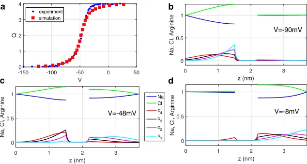
The voltage dependence of the charge (arginines) trans-ferred from intracellular vestibule to extracellular vestibule is characterized as a QV curve in experimental papers, and it is sigmoidal in shape (20). Fig. 2 a shows that our computed QV curve—the dependence of Q3 on V—is in

very good agreement with the experiment (20). This good agreement comes from the fact that our resultant QV curve is also a sigmoidal curve, and, most important of all, the slope of QV curve can be tuned, mainly by the adjustment ofK,KS4, andbS4, to agree with experiment. Not many

theo-retical models can achieve this agreement, especially for the slope. Models in (15,16) show good agreement with exper-iments, whereas a mismatch of slope was reported in (17,18). The voltage dependence of activation has been considered a crucial property of the sodium conductance since it was defined (1). Fig. 2 b shows the steady-state distributions of Naþ, Cl, and arginines in the inside nega-tive, hyperpolarized situation (V ¼ 90 mV). As we can see, all the arginines stay in the intracellular vestibule, and none of the arginines move to the extracellular vestibule (Q3z0).

Fig. 2cshows the situation atV¼ 48 mV, which is the midpoint of the QV curve. As we can see, each vestibule has distributions ofci(i¼1, 2, 3, and 4), resulting in half of the

arginines staying in it (Q3¼2). The center-of-mass position

for each arginine, presented later in Fig. 6, shows that R1 and R2 are in the extracellular vestibule, and R3 and R4

are in the intracellular vestibule. There are almost no argi-nines in zone 2 (hydrophobic plug) because of the energy barrier in it. Note that this represents an average because in a single molecule interpretation, half of the sensors will be with all R’s inside and the other half with all R’s outside. The midpoint of48 mV from (20) requires the resting po-sition of S4,ZS4,0, to be biased fromLRþ0.5LtoZS4,0¼

LRþ0.5Lþ1.591 nm; otherwise, the midpoint would be

0 mV. Fig. 2 d shows the situation at full depolarization (V¼ 8 mV), at which time all arginines move to the extra-cellular vestibule (Q3z 4) in the fully depolarized,

acti-vated state.

Gating current

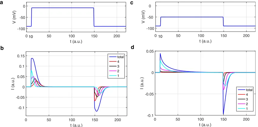
Fig. 3shows the time course of gating currents, observed as flux of charge at the middle of hydrophobic plug

I(LRþL/2,t) because of the movement of arginines when

the membrane depolarization is large and when the depolar-ization is small. In the case of large depolardepolar-ization,Vrises from 90 mV at t ¼ 10 to 8 mV and drops back to 90 mV att¼150 (Fig. 3a). The time course of gating cur-rent and contributions of individual arginines are shown in

Fig. 3 b. As expected, the rising order of each current component follows the moving order of R1, R2, R3, and R4 when depolarized and that order is reversed when repo-larized. The area under the gating current is the amount of charge moved. Because arginines move forward and back-ward in this depolarization/repolarization scenario, the areas under the ON current and the OFF current are same. The areas are equal for each component of current as well. The equality of area is an important signature of gating current that contrasts markedly with the properties of ionic current (26,27). In the case of small depolarization (Vrises from90 to50 mV att¼10 to and drops back to90 mV att¼150,Fig. 3c), the time course of gating current and its four components contributed by each arginine for this situ-ation is shown inFig. 3d. Under this small depolarization, not all arginines move past the middle of the hydrophobic

-150 -100 -50 0 50

V 0 1 2 3 4 Q a experiment simulation

0 1 2 3

z (nm) 0

0.5 1

Na, Cl, Arginine

b Na Cl c4 c₃ c2 c₁

0 1 2 3

z (nm) 0

0.5 1

Na, Cl, Arginine

c

0 1 2 3

z (nm) 0

0.5 1

Na, Cl, Arginine

d

V=-90mV

V=-48mV V=-8mV

FIGURE 2 (a) QV curve and comparison with (20). Steady-state distributions for Naþ, Cl, and arginines are shown at (b) V ¼ 90 mV, (c)V¼ 48 mV, and (d)V¼ 8 mV. Note that the experimental data in (20) were scaled to 4e. To see this figure in color, go online.

Horng et al.

plug because of the weaker driving force in the small depo-larization compared with the large depodepo-larization case. This can be inferred because the areas under each component current are different (Fig. 3d).

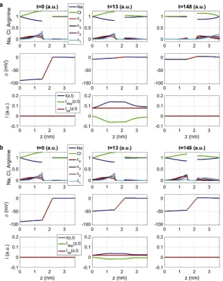
The gating currents can be better understood by looking at a sequence of snapshots showing the spatial distribution of electric potential, species concentration, and electric current. The distributions at several times are shown in

Fig. 4afor the case of sudden change in command voltage to a more positive value and a large depolarization, and the distributions are shown in Fig. 4b for the case of a small depolarization. The electric potential profiles at t ¼ 13 and t ¼ 148 show that the profile of electric potential changes as arginines move from left to right even though the voltage is maintained constant across the sensor. Slight bulges in electric potential profile exist wherever arginines are dense. This can be easily explained by understanding the effect ofEq. 1on a concave spatial distribution of elec-tric potential.

In Fig. 4, the total current defined in Eq. 11, though changing with time, is always constant inzat all times, satis-fying Kirchhoff’s law (i.e., conservation of current). At

t ¼ 13, when gating current is substantial, as seen from

t¼13 inFig. 3,bandd, we can visualize thezdistributions of flux of chargesI(z,t), displacement of currentIdisp(z,t),

and total currentItot(z,t) individually inFig. 4.

Flux of charges at different locations

Flux of charges I(z,t), together with displacement current

Idisp(z,t) and total currentItot(z,t), depicted inFig. 4, deserve

more discussion here. ThoughI(z,t),Idisp(z,t), andItot(z,t) are

well defined inEqs. 8,9,10, and11, the actual computation of them takes an indirect path because of the assumption of qua-sisteady state for Naþand ClinEq. 2. The details are pre-sented in Supporting Materials and Methods, Section S9. The computed total current Itot(z, t) does indeed satisfy

Kirchhoff’s law by its uniformity inz. This verification is shown inFig. 4at several times, and we have checked that this is in fact true at any time.

In the bottom rows ofFig. 4att¼13, we observe that

I(z,t) is generally nonuniform in zand is accompanied by congestion/decongestion of arginines in between. However,

I(z,t) is almost uniform in zone 2 (hydrophobic plug), which means almost no congestion/decongestion of arginines oc-curs there, and therefore, there is no contribution to the displacement current d=dtQnetðz;tÞ from zone 2. This is

because arginines can hardly reside in zone 2 because of the energy barrier in it.

Several things are worth noting in the time courses of

IðLRþL=2;tÞ and I(0, t) (equal to uniformly distributed

Itotas depicted byEq. 11) illustrated inFig. 5a under the

case of large depolarization. First,IðLRþL=2;tÞis

notice-ably larger thanI(0,t) in the ON period. This is because their difference, exactly the displacement currentIdisp, is always

negative at zone 2 when depolarized because arginines are leaving zone 1 and make d=dtQnet < 0 for zone 2.

It is expected that the area under the time course of

IðLRþL=2;tÞ would be very close to 4e, as verified

by the time courses ofQ3inFig. 5b. We useI(0,t) to

esti-mate the experimentally measured voltage-clamp current, whereas the counterpart area of experimentally measurable

I(0,t) would be less than 4e because of its smaller magni-tude compared withIðLRþL=2;tÞ. This may partly explain

0 50 100 150 200

t (a.u.) -0.1 -0.05 0 0.05 0.1 0.15 I (a.u.) total 4 3 2 1

0 50 100 150 200

t (a.u.)

-100 -50 0

V (mV)

0 50 100 150 200

t (a.u.)

-0.1 -0.05 0 0.05

I (a.u.) _total

4 3 2 1

0 50 100 150 200

t (a.u.) -100 -50 0 V (mV) a b c d 10 10

FIGURE 3 (a) The time course ofVrising from90 to8 mV att¼10 holds on untilt¼150 and then drops back to90 mV. (b) The time course of gating current,I(LRþL/2,t), and its components corresponding to (a) are shown. (c) The time course ofVrising from90 to50 mV att¼10 holds on until

t¼150 and then drops back to90 mV. (d) The time course of gating current,I(LRþL/2,t), and its components corresponding to (c) are shown. To see this figure in color, go online.

Gating Currents Model

the experimental observations that at most 13e (25,28,29), instead of 16e, are moved during full depolarization in four voltage sensors (for a single ion channel) based on computing the area under voltage-clamp gating current. Therefore, flux of charge at any location of zone 2, though impossible to measure in experiments so far, will give us the amount of arginines moved during depolarization more reliably than the measurableI(0,t).

Second, we see inFig. 5awith magnification in its inset plot that, as in experiments,I(0,t), but notIðLRþL=2;tÞ, has

contaminating leading spikes in ON and OFF parts of the current. These spikes are capacitive currents from solution EDL of vestibules caused by the sudden rising and dropping of command potential. These spikes need to be removed in voltage-clamp experiments to get rid of the contribution from vestibule solution EDL (and membrane) to the trans-port of gating charges (arginines) when computing the area under gating current. The technical details of removing these spikes are shown in Supporting Materials and

Methods, Section S10, and more details about spikes can be found inSupporting Materials and Methods, Section S11. Third, inFig. 5b, as arginines move from one vestibule to another, the concentrations of Naþand Clalso corre-spondingly change with time at the vestibules. They form countercharges through EDL and balance arginine charges at vestibules. However, these EDL changes only maintain an approximate, not exact, charge balance, as shown in

Fig. 5 b. The violation of electroneutrality causes the displacement current, which is not negligible. This further causes the underestimate of arginines that move when the voltage sensor is depolarized if the estimate is made by measuring the area underI(0,t).

As in the previous section, we used flux of charges at the middle of the hydrophobic plug,I(LR þL/2, t), instead of

experimentally measurable I(0, t) to represent the gating current in discussions. We may as well name I(LR þ

L/2, t) as the arginine current to avoid the confusion with the actual gating currentI(0,t) here. This arginine current

FIGURE 4 (a) The top row shows dimensionless species concentration distributions at t ¼ 0, 13 (right after depolarization), and 148 (right before repolarization) for the case of large depolarization withVfrom90 mV att¼10 to8 mV and drop-ping back to 90 mV at t ¼ 150. The middle row shows concurrent electric potential profiles. The bottom row shows concurrent electric current profiles with the components of flux of charge, displacement current, and total current. (b) The same as (a) is shown except withVdepolarized from90 to50 mV. To see this figure in color, go online.

Horng et al.

leaves out its associated displacement current Idisp(LR þ

L/2,t) and serves to represent gating current better for two reasons:

1) The area under the time course ofI(LRþL/2,t) gives us

the amount of arginines moved during depolarization more faithfully than I(0, t). The fluxes of charge for each arginine shown inFig. 3,banddcarry important information about how each arginine is moved by the electric field that will be further illustrated in Fig. 6. All these will not be easy to display and comprehend if we useI(0,t) instead.

2) Using I(0, t) as a definition of gating current would require a decontamination by removing the leading spikes, which is computationally costly. Removing spikes would especially pose a heavy numerical burden when doing parameter fitting in which numerous repeated computations are done.

Time course of arginine and S4 translocation

Fig. 6 shows the time course of Q (amount of arginines moved to extracellular vestibule, equal toQ3here) and

cen-ter-of-mass trajectories of individual arginines (zi,CM,i¼1,

2, 3, and 4) and S4 segment (ZS4).Fig. 6,aandbshow the

case of large depolarization, andFig. 6,canddshow the case of small depolarization.

In the case of large depolarization (Fig. 6 b), the argi-nines and S4 z positions quickly reach individual steady states, with almost all arginines transferred to the extracel-lular vestibule as previously shown inFig. 4a. Therefore,

Qis close to its saturated value 4 as shown inFig. 6a. Ar-ginines and S4 move back to the intracellular vestibule once the voltage drops back to90 mV. FromFig. 6b, the for-ward-moving order of arginines is R1, R2, R3, and R4, and the backward-moving order is the opposite R4, R3, R2, and R1 with agreement with the structure. This agreement might look trivial in molecular dynamics simulations but is not a trivial check here because this model describes arginines not by particles, as in molecular dynamics, but by concentrations. Note that an incorrect order and pace of the movement of arginines would cause disagreement with experiments in the shape of IV curve as well. S4 is initially farthest to the right but lags behind R1 and R2 dur-ing movement in depolarization, as shown inFig. 6b. This is certainly because S4 is finally relaxed to an almost unforced situation close to its resting positionZS4,0during

a

b

FIGURE 5 (a) The time courses ofIðLRþL=2;tÞ, I(0,t), and despikedI(0,t) for the case of large depo-larization withVrising from90 to8 mVatt¼10, holding on till t¼ 150, and then dropping back to 90 mV. The inset plot is a magnification of the ON current to visualize the difference of

I(0,t) and despikedI(0,t) more clearly. (b) The time courses of Q1; Q3; R0LRðcNa cClÞdz, and R2LRþL

LRþL ðcNacClÞdzare under the same

depolariza-tion scenario as (a). To see this figure in color, go online.

0 50 100 150 200

t (a.u.) 0

2 4

Q

0 50 100 150 200

t (a.u.) 0

1 2

Q

0 50 100 150 200

t (a.u.) 1 2 3 zi,CM , z S4 (nm) z_4,CM z 3,CM z 2,CM z_1,CM z S4

0 50 100 150 200

t (a.u.) 0.5 1 1.5 2 2.5 3 zi,CM , z S4 (nm) z_4,CM z 3,CM z_2,CM z_1,CM z S4 a c d b

FIGURE 6 (a) and (c) are the time courses of the amount of arginines moved to the extracellular vestibule. (b) and (d) are center-of-mass trajec-tories of individual arginines and S4. (a) and (b) are the case of large depolarization withVrising from90 to8 mV at t¼ 10, holding on till

t ¼ 150, and then dropping back to 90 mV. (c) and (d) are the case of small depolarization withVrising from90 to50 mV att¼10, hold-ing on tillt ¼150, and then dropping back to

90 mV. To see this figure in color, go online. Gating Currents Model

this large depolarization. We can further calculate the displacements of each arginine and S4 during this full-saturating depolarization and find Dz1,CM z Dz2,CM z Dz3,CM z 1.93 nm, Dz4,CM ¼ 1.76 nm, and DZS4 ¼

1.51 nm. Besides almost the same displacements for R1, R2, and R3, their average moving velocities are also very close to each other. This seems to suggest a synchronized movement among R1, R2, and R3 that we have not imposed on the arginines in our model. Also, we can see the move-ments of arginines contribute significantly to the movement of the S4 segment. This can be seen from the steady-statez

position of S4 derived fromEq. 6,

ZS4 ¼ K KS4þ4K

X4

i¼1

ðzi;CMziÞ þ KS4

KS4þ4K ZS4;0

¼ 1₅

"

ZS4;0þ

X4

i¼1 zi;CM

#

: (11)

Experimental estimates of S4 displacement during full de-polarization range from 2 to 20 A˚ (24,30), depending on the model of the voltage sensor and its motion, including the transporter model, the helical screw, and the paddle model (24). OurDZS4¼1.51 nm here is large and seems to agree

better with experimental estimates requiring large displace-ments, such as the paddle model. In contrast, the helical screw model, which is supported by most of the recent data, is known to have shorter displacements. A plausible explanation for our overestimate ofDZS4is that our 1D model

uses a straight line perpendicular to the hydrophobic-plug path for the movement of the arginines. In reality, the S4 segment is significantly tilted with respect to the membrane, and the arginines follow a spiral along the helix. Therefore, if the S4 segment rotates and changes its tilt during activation, the total vertical translation needed to cross the hydrophobic plug is significantly reduced, as was shown by Vargas et al.

(31). The value obtained in (31) was between 0.7 and 1 nm when comparing the displacement perpendicular to the mem-brane of the open-relaxed state crystal structure of Kv1.2 (32) and the closed structure that has been derived by consensus from experimental measurements (31).

In the case of small depolarization, the driving force is weaker than in a large-saturating depolarization, so their

zpositions do not have a chance to reach steady states as they do during a full-saturating depolarization. Rather, in a small depolarization, the motion of the arginines and S4 are aborted. They return to the intracellular vestibule because the depolarization drops (i.e., decreases in magni-tude, and the membrane potential becomes more negative) before arginines and S4 have a chance to reach their steady-state positions. This detailed atomic interpretation likely overreaches the resolution of our model. At the sin-gle-sensor level, we do not expect partial movements; instead, some sensors will have moved all the way and others not at all, but the distribution of sensors in the two extreme positions should follow what we predict with this model, which is an ensemble average. We look forward to measurements of movements of probes that mimic arginine in its environment that require improvements in the resolu-tion and structural realism of our model.

Fig. 6cillustrates these aborted motions.Qreaches 1.57 at most, which should be 2 instead if steady-state was reached as it is if time is long enough. See the steady-state behavior shown in the QV curve ofFig. 2a.Fig. 6dshows that the S4 segment is initially farthest to the right, lags behind R1 during movement, and is almost caught up by R2. The maximal displacements of arginines and S4 calcu-lated from Fig. 6 d are Dz1,CM ¼ 1.36 nm, Dz2,CM ¼

0.966 nm,Dz3,CM ¼ 0.459 nm, Dz4,CM ¼ 0.316 nm, and DZ4,CM ¼ 0.616 nm. The significant difference between Dz1,CM, Dz2,CM, Dz3,CM, and Dz4,CM may imply that R1

and R2 have jumped across the hydrophobic plug and entered the extracellular vestibule, whereas R3 and R4

a b

FIGURE 7 (a) The time courses of subtracted gating current, despikedI(0,t), with the voltage rising from90 toVmV att¼10, holds on till

t¼150, and then drops back to90 mV, where

V ¼ 62, 50, ., 8 mV. (b) t2 versus V

compared with experiment (20) is shown. To see this figure in color, go online.

Horng et al.

still stay at the intracellular vestibule during this small depolarization. This is consistent with the observation from individual gating-current components of arginines in

Fig. 3d.

Family of gating currents for a range of voltages

Though we prefer IðLRþL=2;tÞtoI(0,t) for representing

gating current as explained in the section under heading

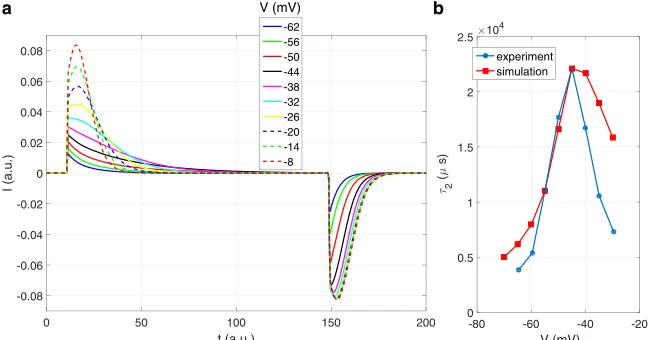
Flux of Charges at Different Locations, we here use the actual gating current, despiked I(0, t), to compare with experiment (20).Fig. 7a shows the time courses of a sub-tracted gating current (despikedI(0,t)) for a range of volt-ages V ranging from 62 to 8 mV. The area under gating current, for both ON and OFF parts, increases withVbecause more arginines are transferred to the extra-cellular vestibule asVincreases. The shapes of this family of gating currents agree well with experiment (20) in both magnitude and time course.

We can characterize the time course by fitting the decay part of a subtracted gating current by aet=t_{1þ be}t=t_2, t1<t2as generally done in experiments (20) in whicht1 is the fast time constant and t2is the slow time constant. Usually, the movement of arginines is dominated by t2. Here, t2 was calculated from simulation and compared with experiment (20) as shown inFig. 7b. Because in our computation the time is in arbitrary units, we have scaled the time to have the maximalt2to fit with its counterpart in experiment (20). Overall, the trend oft2versusVin our result, though not the whole curve, agrees well with exper-iment (20). To the left of the maximal point in Fig. 7 b, simulation results fit rather well with the experiment compared with the values to the right of the maximal point, at which it overestimatest2compared with the experiment. This overestimate is consistent with the observation that the amount of transferred chargesQsaturates slightly faster in experimental data than in this simulation as V increases (see QV curve of Fig. 2 a). This phenomenon is related

to the cooperativity of movement among arginines, which will be further discussed below.

Effect of voltage pulse duration

Fig. 8shows the effect of voltage pulse duration withFig. 8a

for the case of small depolarization andFig. 8bfor the case of large depolarization. The magnitude and time span of sub-tracted gating current (despikedI(0,t)) are changed by pulse duration in both cases, but the shape will asymptotically approach the same curve as pulse duration increases, no matter the size of the depolarization. This behavior occurs because it takes time for the command pulse to drive the ar-ginines toward the extracellular vestibule. If the pulse dura-tion is long enough, the time course ofQwill approach its steady state for large depolarization as inFig. 6a. Small de-polarization takes a longer time to reach its steady state, as demonstrated inFig. 6 c. The shapes of gating currents in

Fig. 8 compare favorably with experiment (20) in which the OFF subtracted gating currents for short pulses have very fast decays, whereas for long pulses, the OFF subtracted gating currents have larger rising amplitude and slower decay because of a larger amount of arginines moved.

CONCLUSIONS

Previous work with molecular and coarse-grained simula-tions have captured some interacsimula-tions, but they have not yet reproduced the time course and voltage dependence of macroscopic gating currents (10–14), and previous contin-uum models have captured only the steady-state properties of charge movement (15–18).

This 1D continuum mechanical model of the voltage sensor tries to capture the essential structural details of the movement of mass and charge that are necessary to repro-duce the basic features of experimentally recorded gating currents. After finding appropriate parameters, we find that the general kinetic and steady-state properties are

0 20 40 60 80 100 120 140 160 180

-0.1 -0.05 0 0.05

I (a.u.)

0 20 40 60 80 100 120 140 160 180

t (a.u.) -0.1 0 0.1 I (a.u.) a b

FIGURE 8 Subtracted gating currents, despiked

I(0,t), showing the effect of voltage pulse duration. (a)Vincreases from90 to35 mV att¼10 and drops back to90 mV at various times. (b)V in-creases from90 to 0 mV att ¼10 and drops back to90 mV at various times. To see this figure in color, go online.

Gating Currents Model

well represented by the simulations. The good agreement of our numerical results with salient features of gating current measured experimentally would be impossible by simply tuning of parameters if our model had not captured the essence of physics for the voltage sensor. The continuum approach seems to be a good model of voltage sensors, pro-vided that it 1) takes into account all interactions crucial to the movement of gating charges and S4; 2) computes their correlations consistently, so all variables satisfy all equa-tions under all condiequa-tions with one set of parameters; and 3) satisfies conservation of current. This last point gave us a new insight: what is measured experimentally does not correspond to the transfer of the arginines because the total current, containing a displacement current, is smaller than the arginine current. It should be noted, how-ever, that the total energy provided by the voltage clamp isqV, whereq is the time integral of the measured gating current andVis the applied voltage. This is the total energy that explains the correspondence of charge per channel with the charge estimated by the limiting slope method (33–35). We have simplified the profile of the energy barrier in the hydrophobic plug because the PMF in that region, and its variation with potential and conditions, is unknown. There is plenty of detailed information on the amino acid side chains in the plug and how each one of them changes the ki-netics and steady-state properties of gating charge move-ment (6). Therefore, the next step is to model the details of interactions of the moving arginines with the wall of the hydrophobic plug and the contributions from other sur-rounding charged protein components. Some of the effects to be included are as follows:

1) Steric and dielectric interactions of the arginines that this model does not include. These include the interaction of arginines with negative charges of the S2 and S3 seg-ments and the negative phospholipids as well as the hy-drophobic residues in the plug. These interactions may be responsible for the simultaneous movement of two to three arginines across the plug, which is an experi-mental result that this model does not reproduce (36,37). 2) Time dependence of the plug energy barrierVb.Once the

first arginine enters the hydrophobic plug by carrying some water with it, this partial wetting of the hydropho-bic plug will lowerVb, chiefly consisting of solvation

en-ergy, and enable the next arginine to enter the plug with less difficulty. This might explain the cooperativity of movement among arginines when they jump through the plug. The addition of details in the plug may also pro-duce intermediate states that have been measured exper-imentally. In this situation, arginines may transiently dwell within the plug.

3) A very strong electric field might affect the hydration equilibrium of the hydrophobic plug and would lower its hydration energy barrier as well (38). This cooper-ativity of movement may help explain the quick

satura-tion in the upper right branch of the QV curve (and smaller t2). It may also explain the experimentally observed translocation of two to three arginines simulta-neously (36,37).

The power of this mathematical modeling is precisely the implementation of interactions and the various effects in a consistent manner. Implementing the various effects listed above is likely to lead to a better prediction of the currents and to the design of experiments to further test and extend the model.

Further work must address the mechanism of coupling between the voltage sensor movements and the conduction pore. For example, the spring constant of the two sides of S4 have been made equal, which does not take into account the structural reality that one side has a linker to S3, whereas the other links to the pore opening. It seems likely that the classical mechanical models of coupling will need to be extended to include coupling through the electrical field. The charges involved are large. The distances are small, so the changes in electric forces that accompany movements of charged mass (and flows of displacement current) are likely to be large and important. It is possible that the voltage sensor modifies the stability of a funda-mentally stochastically unstable, nearly bistable, conduc-tion current (of single channels) by triggering sudden transitions from closed to open state in a controlled process reminiscent of Coulomb blockade in a noisy environment (39).

SUPPORTING MATERIAL

Supporting Materials and Methods, one figure, and one data file are avail-able at http://www.biophysj.org/biophysj/supplemental/S0006-3495(18) 34501-6.

AUTHOR CONTRIBUTIONS

All authors conceived the research, T-L. H. wrote the code and carried out the computations, and all authors contributed to the interpretation and writing of the manuscript.

ACKNOWLEDGMENTS

Dr. Horng thanks the support of National Center for Theoretical Sciences Mathematical Division of Taiwan and Dr. Ren-Shiang Chen for the long-term helpful discussions.

This research was sponsored in part by the National Institutes of Health grant R01GM030376 (F.B.), National Science Foundation Division of Mathematical Sciences grant 1759535 (C.L.), National Science Foundation Division of Mathematical Sciences grant 1759536 (C.L.), and Ministry of Science and Technology grant 106-2115-M-035-001-MY2 (T.-L.H.).

SUPPORTING CITATIONS

References (40–51) appear in theSupporting Material. Horng et al.

REFERENCES

1. Hodgkin, A. L., and A. F. Huxley. 1952. A quantitative description of membrane current and its application to conduction and excitation in nerve.J. Physiol.117:500–544.

2. Feynman, R. P., R. B. Leighton, and M. Sands. 1963. The Feynman Lectures on Physics, Vol. 2: Mainly Electromagnetism and Matter. Ad-dison-Wesley, New York.

3. Jimenez-Morales, D., J. Liang, and B. Eisenberg. 2012. Ionizable side chains at catalytic active sites of enzymes.Eur. Biophys. J.41:449–460. 4. Eisenberg, B., Y. Hyon, and C. Liu. 2010. Energy variational analysis of ions in water and channels: field theory for primitive models of com-plex ionic fluids.J. Chem. Phys.133:104104.

5. Horng, T. L., T. C. Lin,., B. Eisenberg. 2012. PNP equations with steric effects: a model of ion flow through channels. J. Phys. Chem. B.116:11422–11441.

6. Lacroix, J. J., H. C. Hyde,., F. Bezanilla. 2014. Moving gating charges through the gating pore in a Kv channel voltage sensor.

Proc. Natl. Acad. Sci. USA.111:E1950–E1959.

7. Zhu, F., and G. Hummer. 2012. Drying transition in the hydrophobic gate of the GLIC channel blocks ion conduction.Biophys. J. 103: 219–227.

8. Schuss, Z., B. Nadler, and R. S. Eisenberg. 2001. Derivation of Poisson and Nernst-Planck equations in a bath and channel from a molecular model.Phys. Rev. E Stat. Nonlin. Soft Matter Phys.64:036116. 9. Schuss, Z. 2009. Theory and Applications of Stochastic Processes: An

Analytical Approach. Springer, New York.

10. Khalili-Araghi, F., V. Jogini,., K. Schulten. 2010. Calculation of the gating charge for the Kv1.2 voltage-activated potassium channel.

Biophys. J.98:2189–2198.

11. Pathak, M. M., V. Yarov-Yarovoy,., E. Y. Isacoff. 2007. Closing in on the resting state of the Shaker K(þ) channel.Neuron.56:124–140. 12. Machtens, J. P., R. Briones,., C. Fahlke. 2017. Gating charge

calcu-lations by computational electrophysiology simucalcu-lations.Biophys. J.

112:1396–1405.

13. Treptow, W., M. Tarek, and M. L. Klein. 2009. Initial response of the potassium channel voltage sensor to a transmembrane potential.

J. Am. Chem. Soc.131:2107–2109.

14. Kim, I., and A. Warshel. 2014. Coarse-grained simulations of the gating current in the voltage-activated Kv1.2 channel. Proc. Natl. Acad. Sci. USA.111:2128–2133.

15. Islas, L. D., and F. J. Sigworth. 2001. Electrostatics and the gating pore of Shaker potassium channels.J. Gen. Physiol.117:69–89.

16. Lecar, H., H. P. Larsson, and M. Grabe. 2003. Electrostatic model of S4 motion in voltage-gated ion channels.Biophys. J.85:2854–2864. 17. Peyser, A., and W. Nonner. 2012. The sliding-helix voltage sensor:

mesoscale views of a robust structure-function relationship.Eur. Bio-phys. J.41:705–721.

18. Peyser, A., and W. Nonner. 2012. Voltage sensing in ion channels: mesoscale simulations of biological devices.Phys. Rev. E Stat. Nonlin. Soft Matter Phys.86:011910.

19. Lin, T. C., and B. Eisenberg. 2014. A new approach to the Lennard-Jones potential and a new model: PNP-steric equations. Commun. Math. Sci.12:149–173.

20. Bezanilla, F., E. Perozo, and E. Stefani. 1994. Gating of Shaker Kþ channels: II. The components of gating currents and a model of channel activation.Biophys. J.66:1011–1021.

21. Eisenberg, B. 2016. Conservation of current and conservation of charge.https://arxiv.org/abs/1609.09175.

22. Eisenberg, B. 2016. Maxwell matters. https://arxiv.org/pdf/1607. 06691.

23. Eisenberg, B., X. Oriols, and D. Ferry. 2017. Dynamics of current, charge, and mass.Mol. Based Math. Biol.5:78–115.

24. Tombola, F., M. M. Pathak, and E. Y. Isacoff. 2006. How does voltage open an ion channel?Annu. Rev. Cell Dev. Biol.22:23–52.

25. Bezanilla, F. 2008. How membrane proteins sense voltage.Nat. Rev. Mol. Cell Biol.9:323–332.

26. Schneider, M. F., and W. K. Chandler. 1973. Voltage dependent charge movement of skeletal muscle: a possible step in excitation-contraction coupling.Nature.242:244–246.

27. Bezanilla, F., and C. M. Armstrong. 1976. Properties of the sodium channel gating current. Cold Spring Harb. Symp. Quant. Biol.40: 297–304.

28. Schoppa, N. E., K. McCormack,., F. J. Sigworth. 1992. The size of gating charge in wild-type and mutant Shaker potassium channels.

Science.255:1712–1715.

29. Seoh, S. A., D. Sigg,., F. Bezanilla. 1996. Voltage-sensing residues in the S2 and S4 segments of the Shaker Kþchannel.Neuron.16:1159– 1167.

30. Kim, D. M., and C. M. Nimigean. 2016. Voltage-gated potassium chan-nels: a structural examination of selectivity and gating.Cold Spring Harb. Perspect. Biol.8:a029231.

31. Vargas, E., F. Bezanilla, and B. Roux. 2011. In search of a consensus model of the resting state of a voltage-sensing domain. Neuron.

72:713–720.

32. Chen, X., Q. Wang,., J. Ma. 2010. Structure of the full-length Shaker potassium channel Kv1.2 by normal-mode-based X-ray crystallo-graphic refinement.Proc. Natl. Acad. Sci. USA.107:11352–11357. 33. Almers, W. 1978. Gating currents and charge movements in excitable

membranes.Rev. Physiol. Biochem. Pharmacol.82:96–190. 34. Sigg, D., and F. Bezanilla. 1997. Total charge movement per channel.

The relation between gating charge displacement and the voltage sensi-tivity of activation.J. Gen. Physiol.109:27–39.

35. Ishida, I. G., G. E. Rangel-Yescas,., L. D. Islas. 2015. Voltage-depen-dent gating and gating charge measurements in the Kv1.2 potassium channel.J. Gen. Physiol.145:345–358.

36. Conti, F., and W. St€uhmer. 1989. Quantal charge redistributions accom-panying the structural transitions of sodium channels.Eur. Biophys. J.

17:53–59.

37. Sigg, D., E. Stefani, and F. Bezanilla. 1994. Gating current noise produced by elementary transitions in Shaker potassium channels.

Science.264:578–582.

38. Vaitheeswaran, S., J. C. Rasaiah, and G. Hummer. 2004. Electric field and temperature effects on water in the narrow nonpolar pores of car-bon nanotubes.J. Chem. Phys.121:7955–7965.

39. Kaufman, I. Kh., P. V. E. McClintock, and R. S. Eisenberg. 2015. Coulomb blockade model of permeation and selectivity in biological ion channels.New J. Phys.17:083021.

40. Trefethen, L. N. 2000. Spectral Methods in MATLAB. Society for Industrial and Applied Mathematics, Philadelphia, PA.

41. Ascher, U. M., and L. R. Petzold. 1998. Computer Methods for Ordi-nary Differential Equations and Differential-Algebraic Equations. So-ciety for Industrial and Applied Mathematics, Philadelphia, PA. 42. Shampine, L. F., and M. W. Reichelt. 1997. The MATLAB ODE suite.

SIAM J. Sci. Comput.18:1–22.

43. Shampine, L. F., M. W. Reichelt, and J. A. Kierzenka. 1999. Solving index-1 DAEs in MATLAB and simulink.SIAM Rev.41:538–552. 44. Sigg, D., F. Bezanilla, and E. Stefani. 2003. Fast gating in the Shaker

Kþ channel and the energy landscape of activation. Proc. Natl. Acad. Sci. USA.100:7611–7615.

45. Stefani, E., and F. Bezanilla. 1997. Voltage dependence of the early events in voltage gating.Biophys. J.72:131.

46. Stefani, E., D. Sigg, and F. Bezanilla. 2000. Correlation between the early component of gating current and total gating current in Shaker K channels.Biophys. J.78:7.

47. Forster, I. C., and N. G. Greeff. 1992. The early phase of sodium chan-nel gating current in the squid giant axon. Characteristics of a fast component of displacement charge movement. Eur. Biophys. J.

21:99–116.

Gating Currents Model

48. Armstrong, C. M., and F. Bezanilla. 1974. Charge movement associ-ated with the opening and closing of the activation gates of the Na channels.J. Gen. Physiol.63:533–552.

49. Bezanilla, F., and J. Vergara. 1980. Properties of excitable membranes.

In Membrane structure and Function, Volume II, Chapter 2. E. E. Bittar, ed. J. Wiley & Sons, pp. 53–113.

50. Bezanilla, F., and C. M. Armstrong. 1977. Inactivation of the sodium channel. I. Sodium current experiments. J. Gen. Physiol.

70:549–566.

51. Ferna´ndez, J. M., F. Bezanilla, and R. E. Taylor. 1982. Distribution and kinetics of membrane dielectric polarization. II. Frequency domain studies of gating currents.J. Gen. Physiol.79:41–67.

Horng et al.

Biophysical Journal, Volume116

Supplemental Information

Continuum

Gating

Current

Models

Computed

with

Consistent

Interactions

1

1. Non-dimensionalization

We non‐dimensionalize all physical quantities as follows,

̃ , _/ , , ̃ , ̃ _/ , , _/ , _/ ,

,

where is concentration of species i, with i=Na+_{, Cl}_{, 1, 2, 3, and 4. Each is} scaled by which is the bulk concentration of NaCl in the

intracellular/extracellular domains. Here is set to be 184mM, equal on both

sides, so that the Debye length is 1nm when the relative

permittivity 80. is the electric potential scaled by / with

being the Boltzmann constant; the temperature; e the elementary charge. All relevant external potentials U are scaled by . All sizes s are scaled by R, which is the radius of vestibule as shown in Fig. 1(b). R=1nm here. The time t is scaled

by / , with being a diffusion coefficient that can be adjusted later to be

consistent with the time spans of on/off currents measured in experiments (caused by the movement of arginines). The diffusion coefficient of species i is

scaled by . The coupling constant of PNP‐steric model based on

combining rules of Lennard Jones, representing the strength of steric interaction between species i and j, is scaled by / [1,2].For simplicity, we assume

, for all

0, for all , , 1,2,3,4. Note that here we only consider steric interaction among arginines. We think they are a crucial source of correlated structural change and motion (of mass and charge). The consideration of steric effect among arginines is justified by the fact that arginines are generally crowded in hydrophobic plug and vestibules. The flux density of speciesi, , is

scaled by / , and therefore the electric current I is scaled by . For

simplicity of notation, we will drop ~ for all dimensionless quantities shown in all equations.

2.Shapeofpotentialofmeanforce(PMF)inthehydrophobicplug

Here, we simply assume a hump shape for PMF in the hydrophobic plug as,

, tanh 5 tanh 5 1 , when is in zone 2,

0, when is in zone 1 and 3, (S1)

2

Theoretically, if we set , too large, the gating current would be slow and

perhaps small because it would be very difficult for arginines to move across this barrier. The double tanh functions are designed to smooth the otherwise

top‐hat‐shape barrier profile, which is not good for numerical differentiation because of its awkward infinite slopes. This smoothing is simply based on the belief that the energy barrier in a protein structure does not have a jump. In future work, it would be wise to compute the PMF from a specific model of charge distribution (both permanent and polarization) constructed from a combination of structural data and molecular dynamics simulations, if feasible.

3.Governingequationsderivationfromenergyvariationmethods

Governing equations Eqs. (1‐4) were derived by energy variational methods based on the following energy (in dimensional form):

∑ | | ∑ ∑

∑ _, , (S.2)

where the first term is entropy; second and third terms are electrostatic energy; the fourth term is the constraint and barrier potential for arginines; the last term is the steric energy term, based on Lennard‐Jones potential [1,3]. The Poisson equation Eq. (1) is derived from the variation of energy with respect to electric potential

0,

and species flux densities in Eqs. (3,4) are derived by

, ,

where is the chemical potential of species i.

4.Quasi‐steadinessassumptionforNa+_andCl‐

Here we assume quasi‐steady state for Na+ _{and Cl}‐_{, which means 0,}

Na, Cl. The steady state assumption here is justified by the fact that the diffusion coefficients of Na+ _{and Cl} _{in vestibules are much larger than the diffusion}

coefficient of arginine based on the very narrow time span of the leading spike of gating current measured in experiments. The spike comes from the linear

3

calculations.Otherwise using realistic diffusion coefficients for Na+ _{and Cl}‐ _would render Eqs. (1‐4) too stiff to integrate in time. The spike contaminating the gating

current is removed in experiments by a simple technique called P/n leak

subtraction (see Section 11; n typically is 4). P/n leak subtraction is also used to subtract the linear capacity current of all the membranes in the real system that are not included in our model. How to do leak subtraction computationally will be discussed in Section 10.

5.Formulationofboundaryconditions

Types of boundary conditions are illustrated in Fig. 1(b). Note the no‐flux boundary conditions specified in Fig. 1(b). One prevents Na+ _{and Cl} _from

entering the hydrophobic plug (zone 2) with low dielectric coefficient. The other

boundary condition constrains S4 motion and so prevents the arginines from

leaving the vestibules into intracellular/extracellular domains. Boundary and interface conditions for electric potential are

0 , , Γ Γ ,

, Γ Γ

, 2 0. (S.3)

These are Dirichlet boundary conditions at both ends and continuity of electric potential and displacement at the interfaces between zones. Boundary and interface conditions for arginine are

0, 2 , 0, , , , ,

, , , , , ,

, , 1,2,3,4, (S.4) where no‐flux boundary conditions are placed at both ends of the gating pore, consisting of vestibules and hydrophobic plug, to prevent arginines and S4 from

entering intracellular/extracellular domains. The others are continuity of

concentration and flux at interfaces between zones. Boundary conditions for Na+

and Cl are

0, 0, 2 , 2 , 1,

, , , , 0, (S.5)

4

impermeability of Na+ _{and Cl}_{into hydrophobic plug.}

6.Parametersfitting

We have tried and found Di=50, i=1,2,3,4,K=3, KS4=3, bS4=1.5 provide the

best fit to the important experiments reported in [4]. Several things are to be noted about the parameter values specified above: (1) there is no experimental measurement of diffusion coefficient of arginine inside vestibule and plug available that we can use for simulation. Imprecise setting of the values of these diffusion coefficients only affects the scale of time in I‐V curve, but not its shape. That is why we set time coordinate to be in an arbitrary unit later in results, and here we only focus on comparing the shape of IV curves with experiments in [4]. (2) K, KS4, and bS4 were particularly determined by fitting with QV curve in

experiment [4]. The QV curve is very sensitive to K and KS4, and many efforts have

been taken to achieve proper values for them. The method of fitting is done by trial and error. Choosing incorrect K and KS4 would end up serious mismatch of

QV curve with experiment [4] as demonstrated by the case of K=3 and KS4=12 in

Fig. 1 here. The choice of K=3 and KS4=3 fits experiment [4] best and is adopted

for the rest of simulations.

Figure 1. Simulated QV curves under different K and KS4 compared with

experimental counterpart from [4]. Note that the experimental data in [4] was scaled to 4e.

5 andspeciestransportequation

Eq. (8) is consistent with Ampere’s law in Maxwell’s equations:

, (S.6)

or equivalently,

∙ 0, (S.7)

where is the electric field and is flux density of charge (current density). Eq. (S.7) tells us that the total current is conserved everywhere and it consists of flux

of charges and displacement current . Eq. (S.7) can be derived from the

Poisson equation and species transport equation like Eq. (1) and Eq. (2). Starting from Poisson equation in dimensional form:

∙ ∑ , (S.8)

or equivalently

∙ ∑ . (S.9)

Taking time derivative of Eq. (S.9),

∙ ∑ , (S.10)

and using species transport equation based on mass conservation,

∙ 0, (S.11)

then

∙ ∑ ∙ ∑ ∙ , (S.12)

which becomes exactly Eq. (S.7) by defining =∑ . (S.13)

A more general treatment that does not involve assumptions about can be found in [5‐7].

Casting Eq. (S.7) into the present 1D framework by integrating it in space and applying the divergence theorem, we have

,

, 0 , 0, . (S.14)

Comparing with Eq. (11), ,

0 , , , (S.15)

6 8.Numericalmethod

High-order multi block Chebyshev pseudospectral methods are used here

to discretize Eqs. (1‐4) in space [8]. The resultant semi discrete system is then a set of coupled ordinary differential equations in time and algebraic equations (an ODAE system) [9]. The ordinary differential equations are chiefly from Eq. (2), and algebraic equations are chiefly from Eq. (1) and boundary/interface conditions Eqs. (S.3‐S.5). This system is further integrated in time by an ODAE solver (ODE15S in MATLAB (The MathWorks, Natick, MA) [10,11]) together with

appropriate initial condition. ODE15S is a variableordervariablestep (VSVO)

solver, which is highly efficient in time integration because it adjusts the time step and order of integration. High order pseudospectral methods generally provide excellent spatial accuracy with economically practicable resolutions. A

combination of these two techniques makes the whole computation very efficient. This is particularly important here, since numerous computations have to be tried during the tuning of parameters. Efficiency will be vital in future

calculations comparing theory and experiment in a wide variety of mutants and experimental conditions.

9.Computationoffluxofcharge,displacementcurrentandtotalcurrent

According to definition in Eq. (10), flux of charges at the middle of gating

pore, /2, , and both ends of gating pore, 0, and 2 , ,

should be computed by

, ∑ , , (S.16)

0, 0 ∑ , 0, , (S.17)

2 , 2 ∑ , 2 , . (S.18)

Except , , 0, and 2 , are trivially zero due to the

implement of quasi‐steadiness 0, Na, Cl, in vestibules, which causes

and to be uniform in vestibules by Eq. (2), and further become zero by

the no‐flux boundary conditions for Na and Cl at the bottom of vestibules as described in Eq. (S.5). We have to alternatively reconstruct 0, and

2 , by charge conservation of Na and Cl ,

0, ∑ _, , (S.19)

7

After obtaining 0, and 2 , , we can further reconstruct the flux of

charges , at zone 1 and zone 3 by (8) and (9),

, 0, ∑ , ∈ 0, , (S.21)

, 2 , ∑ , ∈ , 2 . (S.22)

Flux of charge at zone 2 is simply

, ∑ , , ∈ , , (S.23)

since Na and Cl are not allowed to enter zone 2, the hydrophobic plug.

10.Removingspikeintotalcurrent

In voltage‐clamp experiments, subtracting this linear capacitive component and removing the spike from gating current is done by ‘leak subtraction’, in various forms, e.g., P/4 (see details in Section 11) In reality, this linear capacitive current that is subtracted in this procedure comes from both the lipid bilayer membrane in parallel with the gating pore. Here, we only considered the capacitive current from solution EDL of vestibule inside the gating pore and

ignored the membrane capacitive current because we simply use Dirichlet boundary conditions for at both ends of the gating pore in Eq. (S.3). Actually, capacitive current of the membrane in parallel with the gating pore would be much larger than vestibule capacitive current. Following the idea of the

experiment [4], we calculated 0, with V rising from ‐150 mV to ‐140 mV at

t=10, and dropping back to ‐150 mV at t=150. We chose from ‐150 mV to ‐140

mV because essentially none of the arginines move across the hydrophobic plug in this hyperpolarized region. The voltage step quickly charges and discharges solution EDL in vestibules, and the computed time course of 0, is just two

spikes at on and off of the command potential. Subtracting this hyperpolarized 0, , multiplied by a proportion factor (due to the linearity of capacitive current), from its original counterpart will then remove the spikes, and the

unspiked 0, is shown in Fig. 5(a). In preliminary calculations with the model, when the command voltage pulse rises faster, the early spike becomes larger and is still visible even after subtraction, suggesting that is the origin of the early transient gating current in experiments [12‐14].

11.Removinglinearcapacitivecurrenttoobtaingatingcurrentin experiments