Statistical process control by quantile approach

Statistical process control by quantile approach.

Available from Sheffield Hallam University Research Archive (SHURA) at: http://shura.shu.ac.uk/19285/

This document is the author deposited version. You are advised to consult the publisher's version if you wish to cite from it.

Published version

ARIF, Osama H. (2000). Statistical process control by quantile approach. Doctoral, Sheffield Hallam University (United Kingdom)..

Copyright and re-use policy

See http://shura.shu.ac.uk/information.html

1 0 1 6 5 7 5 7 5 0

REFERENCE

ProQuest Number: 10694165

All rights reserved

INFORMATION TO ALL USERS

The quality of this reproduction is dependent upon the quality of the copy submitted.

In the unlikely event that the author did not send a com plete manuscript and there are missing pages, these will be noted. Also, if material had to be removed,

a note will indicate the deletion.

uest

ProQuest 10694165

Published by ProQuest LLC(2017). Copyright of the Dissertation is held by the Author.

All rights reserved.

This work is protected against unauthorized copying under Title 17, United States C ode Microform Edition © ProQuest LLC.

ProQuest LLC.

789 East Eisenhower Parkway P.O. Box 1346

Statistical Process Control

b y

Quantile Approach

Osama Hasan Arif

A thesis submitted in partial fulfilment of the requirements of

Sheffield Hallam University

for the degree of Doctor of Philosophy

Abstract

Most quality control and quality improvement procedures involve making assumptions about the distributional form of data it uses; usually that the data is normally distributed. It is common place to find processes that generate data which is non-normally distributed, e.g. Weibull, logistic or mixture data is increasingly encountered.

Any method that seeks to avoid the use of transformation for non-normal data requires techniques for identification of the appropriate distributions. In cases where the appropriate distributions are known it is often intractable to implement.

This research is concerned with statistical process control (SPC), where SPC can be apply for variable and attribute data. The objective of SPC is to control a process in an ideal situation with respect to a particular product specification. One of the several measurement tools of SPC is control chart. This research is mainly concerned with control chart which monitors process and quality improvement. We believe, it is a useful process monitoring technique when a source of variability is present. Here, control charts provides a signal that the process must be investigated.

In general, Shewhart control charts assume that the data follows normal distribution. Hence, most of SPC techniques have been derived and constructed using the concept of quality which depends on normal distribution. In reality, often the set of data such as, chemical process data and lifetimes data, etc. are not normal. So when a control chart is constructed for 3c or R, assuming that the data is normal, if in reality, the data is non­ normal, then it will provide an inaccurate results.

Schilling and Nelson has (1976) investigated under the central limit theory, the effect of non-normality on charts and concluded that the non-normality is usually not a problem for subgroup sizes of four or more. However, for smaller subgroup sizes, and especially for individual measurements, non-normality can be serious problem.

Acknowledgements

I wish to express sincere appreciation to my supervisor, Professor Gopal G. Kanji for his direction, assistance, encouragement and patience during the research's years. My appreciation also goes to the second supervisor, Professor Warren Gilchrist for his valuable comments, discussion and encouragement.

Statistical Process Control by Quantile Approach

Table of Contents

Abstract...2

Acknowledgements...3

Table of Contents...4

Chapter 1 : Introduction...7

1.1 General Overview...7

1.2 On-line SPC...10

1.3 Off-line SPC...10

1.4 Outlines of Thesis...12

Chapter 2: Literature Review for Statistical Process Control...14

2.1 Introduction...14

2.2 Statistical Process Control...15

2.3 Control Chart...16

2.4 Source of Process Variation... 19

2.5 Hypothesis Testing in SPC...20

2.6 Capability Index...20

2.7 Average Run Length (ARL)...26

2.8 Multivariate Control Chart...27

2.9 Mixture distribution...32

2.10 Effect of Non-normality on control chart...32

Chapter 3: Control Chart Methodology for Non-Normal Situation...35

3.1 Introduction...35

3.2 Quesenberry Technique (Q-Chart)...36

3.3 Box-Cox Transformation...40

Chapter 4: Theoretical Development of Quantile Approach... 44

4.1 Introduction... 44

4.2 Quantile Approach... 45

4.3 Quantile Function for Logistic Distribution... 49

4.4 Quantile Function for Exponential Distribution...54

4.5 Quantile Function for Uniform Distribution...56

4.6 Quantile Function for Extreme-value... 59

4.7 Quantile Function for Weibull Distribution...61

4.8 Quantile Function for Power Distribution...6 6 4.9 Quantile Function for Pareto Distribution...69

4.10 Quantile Function for Geometric Distribution...72

4.11 Summary... 75

Chapter 5: An Evaluation of Quantile Control Chart for Non-Normal Situation 76 5.1 Introduction... 76

5.2 Quantile Control Chart for Non-Normal Distribution...78

5.3 Quantile Control Chart for Logistic Distribution...79

5.4 Quantile Control Chart for Exponential Distribution...8 6 5.5 Quantile Control Chart for Extreme-value Distribution...90

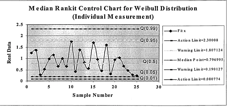
5.6 Quantile Control Chart for Weibull Distribution...91

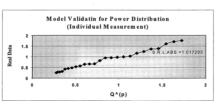
5.7 Quantile Control Chart for Power Distribution...95

5.8 Control chart for non-normal distribution using subgroups of size five... 99

5.9 Summary...103

Chapter 6: Process Capability Indices using Quantile Approach...104

6.1 Introduction...104

6.2 Process capability indices for non-normal distribution...106

6.3 Clement's methods and its weakness...110

6.4 Quantile Approach for Non Normal Capability Indices...112

6.5 Methodology...115

6 . 6 Summary...119

Chapter 7: Determination of Average Run Length (ARL) for Non-Normal Data ....120

7.1 Introduction...120

7.3 ARL for Exponential Distribution... 122

7.4 Application...126

7.5 Summary...138

Chapter 8: Evaluating Multivariate Control Chart using Quantile Approach 140 8.1 Introduction...140

8.2 Multivariate Control Chart using Quantile Approach (MCCQA)...142

8.3 Application...146

8.4 Summary...149

Chapter 9: Quantile Control Chart for Mixture Distribution: AN INNOVATIVE APPROACH...151

9.1 Introduction...151

9.2 Characterisation Theory...153

9.3 Quantile Mixture Distribution...156

9.4 Quantile Control Chart Theory for Mixture Distribution...157

9.5 Application...162

9.6 Summary...166

Chapter 10 Conclusion and Future W ork...168

10.1 Conclusion...168

10.2 Future Work...170

References...172

Appendix...188

Appendix 1...188

Appendix 2...188

Appendix 3...190

Appendix 4...191

Appendix 5... 191

Appendix 6...194

Appendix 7...196

Appendix 8...203

Chapter 1: Introduction

1.1 General Overview

The science of statistics itself goes back only to two or three centuries ago. Its greatest developments have been in the last 70 years. Early applications were not made until the 1920s, that is when theory of statistics began to be applied effectively to quality control. These statistical methods, which investigate the problems of quality control, were first suggested by Walter A. Shewhart of the Bell Telephone Laboratories. In a memorandum prepared on May 16, 1924, he made the first sketch of a modem “control chart”, which he subsequently developed in various memoranda and articles. In 1931 Shewhart published a book on statistical quality control, titled "Economic Control of Quality of Manufactured Product".

Statistics has a very important role to play in the field of manufacturing, covering marketing plan, sales predictions, research and developments, and processes improvement. Statistics is also vital in manufacturing processes, such as incoming quality control, in-process quality control, outgoing quality control, quality assurance, etc. Therefore, statistical understanding plays a major role in product and service quality, care of customers through statistical process control (SPC), customer surveys, process capability and cost of quality etc.

improvement of individuals, groups and organisations. "In order to improve performance, people need to know what to do, how to do it, to have the right tools to do it, to be able to measure performance and to receive feedback on current levels of achievement", (Kanji 1995).

Quality improvement is important and needed for achieving good quality product features with freedom from deficiencies. To maintain and increase sales revenue, companies must continually add new product features and introduce new improved processes to produce such features. Moreover, companies should realise that customers' needs are in a state of change, hence the need to be aware of meeting them. To keep cost competitive, companies must also continually aim at reducing the level of product and process deficiencies. Reduction in production costs besides improving the quality of a product, should be a prime concern to a company, as it would lead to customer satisfaction and consequently arise in sale and profit.

In reality, a company cannot survive in an open market or competitive economy for long if it is not achieving a reasonable level of profits. Such survival would require the company to look for improvement of product and cost reduction in its operations and carry out research and development. There are essential activities for an organisation to take in order to remain competitive and to maintain Business Excellence.

Both techniques have the reduction of variability as their main objective, despite the fact that different methods have been employed to accomplish such an objective. SPC looks for signals representing assignable causes, which may be thought of as external disturbances that increase variability. It also assumes that the process data can be described in terms of statistically independent observations, which fluctuates around a constant mean. On the other hand, EPC actively reverses the effect of process disturbances by making regular adjustments to process variables. EPC is usually discussed in the framework of a process with a drifting mean, and the process adjustments to keep the output quality characteristics on target. EPC accomplishes this basically by transferring variability in the output variable to an input control variable.

The reason why EPC and SPC suggest different strategies for achieving the above mentioned goal, is because of the fact that traditionally they have different processes i.e. two different models. For many engineering systems, it is not only possible to describe them using control behaviour perspective, because they go out of control. This necessitates a form of intervention that will keep such systems in a state of equilibrium, with a small variance. On the other hand, in traditional applications of SPC, it is assumed that in normal conditions the process mean and variance are stable, but abrupt changes in the mean, variance or both, can occur at some unknown moments of time.

Usually, process quality can be improved by reducing output variability, the process failure rate or both.

Statistical process control can be divided into two types. These are on-line SPC and off­ line SPC.

1.2 On-line SPC

On-line SPC methods are technical aid for quality and cost control in manufacturing. On-line SPC consists of preventative and screening processes. In preventative SPC, methods are always preferred, and in which the process itself is being inspected to avoid production of defective items. While, in screening SPC, the output of a process is checked by a system of sampling inspection. Screening helps to provide a basis for making decisions to investigate whether or not to accept the sample batch as satisfactory. This is always an expensive process because it takes more time and money to detect poor performance of the process. Taguchi (1978a) strongly believes that the main objective of an on-line SPC system should be prevention.

1.3 Off-line SPC

Off-line SPC methods are quality and cost control activities conducted at the product and process design stages, in order to improve product manufacturing and reliability, and reduce product development and lifetime costs. Design experiments are a major off­ line SPC tool, because they are often used during activities and the early stages of manufacturing, rather than as a routine on-line procedure.

Taguchi, Elsayed and Hsiang (1989) discussed the robust design approach for determining the optimum configuration of design parameters for performance, quality and cost. The robust design method is an efficient, disciplined approach that can aid product delivery teams in designing for cost. Designing quality with product in mind would prove a cheaper process than trying to inspect and re-engineer such a product, after it hits the production floor, or worse, after it gets to the customer. The robust design method provides a systematic and efficient approach for finding the near optimum combination of design parameters, so that the product is functional, exhibits a high level of performance, and is robust to noise factors. Noise factors are those parameters that are uncontrollable or are too expensive to control.

However, introducing quality at the design stage to improve a process, requires the following overlapping factors:

9 Inspection

9 Quality control « Quality improvement « Quality by design

In order to minimise the effects of noise sources or error in the process, Taguchi suggests that certain counter measures have to be taken for the implementation of the following:

System design the process of applying scientific and engineering knowledge to produce a basic functional prototype design, as in Kackar (1985). The prototype model defines the configuration and attributes of the product undergoing analysis or development. The initial design may be functional, but it may be far from optimum in terms of quality and cost.

Tolerance design the process of determining tolerances around the nominal settings identified in the parameter design process. Tolerance design is required if a robust design cannot produce the required performance without costly special components or high process accuracy.

In this thesis, off-line methods will not be discussed, partly because the aim of the research is to develop and improve quality of product or process through statistical process control using quantile approach. Therefore, the focus of this thesis is on the on­ line preventative SPC on process variable.

1.4 Outlines o f Thesis

This thesis is divided into ten chapters. Chapter one presents a general review of quality control and process control. Process control is divided into two kinds of SPC i.e. on-line SPC and off-line SPC.

Chapter two introduces SPC methodologies, techniques and strategies. It defines control chart under the assumption of normality and discusses the effects of non-normality on control chart, the source of process variation i.e. common cause and assignable (special) cause, Average Run Length (ARL) and the hypothesis test used in SPC. In addition, it reviews the capability index, multivariate control chart and mixture distribution, in normal situation.

Chapter three introduces control chart methodology for non-normal situation and the effect of non-normality on control chart. Some techniques dealing with non-normal situation e.g. Q-chart, Box-Cox transformation are considered. Finally, quantile approach is introduced to deal with the non-normal situation of quality control chart.

Chapter five is dedicated to developing the theoretical aspects of quantile approach, which have been discussed in chapter four, in order to construct quality control charts for non-normal situation.

Chapter six discusses the capability index for non-normal situation, using quantile approach. It also discusses the performance of control charts using average run length (ARL) in chapter seven. Chapter eight, extends the quantile approach to dealing with the multivariate control chart and its applications.

Chapter 2: Literature Review for Statistical

Process Control

2.1 Introduction

The idea of using statistical methods for quality improvement easily extends to the general problems of process improvement. A good way to approach any of these problems is to define performance, measure it, determine the special causes of poor performance, and monitor it, which would result in continuous improvement in quality. Such approaches are generally known as Statistical Process Control (SPC), Carlyle, et al (2000); Montgomery and Woodall (1997).

Statistical Process Control (SPC) have several major tools which can be applied to any process. They are, histogram or stem-and-leaf display, check sheet, pareto chart, cause and effect diagram, defect concentration diagram, scatter diagram and control chart. This research is mainly concerned with control chart which monitors process and improvement. We believe it is a useful process monitoring technique when an unusual source of variability is present, i.e. when the sample average values lie outside the control limits. This provides a signal that the process must be investigated to undertake corrective action

2.2 Statistical Process Control

Statistical process control (SPC) is part of a statistical quality control (SQC), which provides a system of quality control used in place of industrial or other operations.

In addition, one of SPC's major concerns relates to quality management, which is to decrease costs by improving process quality. Usually, process quality can be improved by reducing output variability or the process failure rate, or both. This is in order to quickly detect the occurrence of assignable causes or possible shift, so that investigation of the process and corrective action may be undertaken, before many nonconforming units are manufactured.

Usually, statistical process control uses control charts for monitoring the evolution of a manufacturing process: upper and lower control limits are computed, and if the process operates outside these limits, it is declared out of control and a search for an explanation of this abnormal behavior is initiated. An important tool in statistical process control for finding assignable causes and for monitoring a manufacturing process is the use of the control chart.

2.3 Control Chart

A control chart is a graph of a quality measurement, plotted against time with control lines superimposed to show statistically significant deviations from the normal level of performance. Any significant deviations are assumed to correspond to assignable or special causes, which deserve investigation. A large number of different control charts are discussed in the literature. Each of these charts has the same underlying format but embodies a different statistical model. Control charts can be used for two main purposes. Firstly, it gives an indication of how the level of performance varies with time. Secondly, it monitors improvement, (Wood 1995). Control charts are the basic statistical tools used to monitor and control processes. They can be easily constructed, visualised and interpreted.

methods have been proposed to improve sensitivity to small and moderate sized shifts in the mean. In particular, runs rules have been used to signal for other unusual patterns on the chart, such as having eight sample means in a row either all above or all below the centreline. Runs rules improve the sensitivity, but also increase the number of false alarms. Some of these run rules, which are useful with an J chart in detecting a small sustained shift in the mean, such are rule 1-of-l, rule 2-of-3, rule 4-of-5, rule 9-of-9 an so on, For more details, see Nelson (1984) and Lucas and Saccucci (1990).A typical Shewart control chart is shown in figure 2.1.

U p p er C ontrol Limit

In-C ontrol P oints

Central C ontrol Limit

Low er C ontrol Limit O u t-of-con trol poin;

0 5 10 15

S a m p l e N u m b e r

Figure 2.1 Shewhart Control Chart

In practice, Shewhart charts have been widely used for process monitoring because of an interest in involving production operators in quality improvement and the feeling that they cannot be trained to use other charting methods. Lucas (1976), Crowder (1987) and Lucas and Saccucci (1990) have shown that CUSUM and EWMA charts provide faster detection of small step changes than a non-modified Shewhart chart without an increase in the false-alarm rate.

control limits should be based on a short-term estimate of the process variability, such as the moving average, rather than a long-term estimate, such as sample standard deviation of the process.

The primary purpose of a control chart is thus to quickly detect whenever a change has occurred in a process resulting in an alteration in the mean value or in the dispersion. Control charts may be used to estimate the parameters of a production process and process capability through this estimate. The control chart may also provide useful information for improvement of the process. The eventual goal of statistics process control is the elimination of variability in the process. It may not be possible to completely eliminate variability, but the control chart is an effective tool in reducing variability as much as possible.

In application of statistical method to quality engineering, it is very important to classify data on quality characteristics as either variable or attribute data. Attributes data are usually discrete measurement, often taken the form of counts. On the other hand, variable data are usually continuous measurement, such as length of stay. Most of the work in this thesis will dealing with variable data.

2.4 Source o f Process Variation

A control chart is a statistical tool used to study and control repetitive processes in industrial setting. Shewhart control charts developed to help distinguish between variation in manufacturing that is intrinsic to the production system and variation which is due to external factors. In many production processes, there are many small sources of variation that are inherent in the system itself, which are summarised under the name chance (common) variation. In addition, there is variation that is relatively large and can be assigned to a particular cause, and this is called assignable (special) variation.

A system that only exhibits chance variation is said to be in statistical control; otherwise, it is out of control. There are many types of control charts for different situations, such as individual control charts, x-bar control charts etc. Control charts have upper and lower control limits, often placed three standard deviations from the average. If an observation falls outside these limits, it is considered to be a signal that the process is not in control. These upper and lower control limits are based on estimates of the mean and variance of the process when it is in statistical control.

The ability to separate special/common cause of variations within a process, has enabled management to analyse data and take the necessary actions to improve quality and productivity, at economical cost levels. The basis of such improvement, however, is in the selection, application and interpretation of statistical data generated through the use of the correct type of control charts, (Patel, 1993).

A widely used process indicator is its output distribution characterised by the mean and variance. If the values of means and variance are within prescribed limits, the process is operating in an in-control state. An assignable cause of variability may result in a shift in mean or variance or both, to an out of control state, and thus lead to a defective product, (Chen, 1996).

presence of an assignable cause, an effort is made to find and remove it from the process, if this action is to reduce variability or improve quality. It is also important to detect improvements in process performance, (Woodall and Montgomery, 1999).

2.5 Hypothesis Testing in SPC

There is a connection between hypothesis testing and control charts. Suppose that the vertical axis in figure 2.1 is the sample average (process, say). If the process points lie between the control limits, we conclude that the process mean is in-control and the processes have the same mean and average over time. On the other hand, if the process points exceed control limits, then we conclude that the process mean is out-of-control. It indicates that the process being monitored by SPC control chart, does not have the same mean and variance over time. There is significant evidence that the process is not in- statistical control. Two kinds of error can be occur in testing hypotheses, the first is commonly called a type I error (a) , which occurs, if the null hypotheses rejected when it is true. The second error called a type II error (ft), it takes place, if the null hypotheses is not rejected when it is false. In quality control studies, a is called the producer's risk and p is called the consumer's risk.

2.6 Capability Index

The concept of process capability was introduced by Juran et al. (1974), but did not gain considerable acceptance until the early 1980s. The concept enhances the idea of achieving a process output with minimal variation centred at a target value. Juran realised that there was a need in industry for the development of a single ratio or index, in order to compare the specification interval with the actual process variation.

USL — LSL

Therefore, Juran defined the first process capability index C as C = ---,

6a

where USL and LSL are the Upper and Lower specification limits, respectively, and a

Juran & Gryna (1993) and Montgomery (1997) suggested that the purposes of Process Capability are to:

« Meet or exceed the customer need.

• Predict how well the process will hold the tolerances.

9 Assist product developers/designers in selecting or modifying a process. • Assist in establishing an interval between sample for process monitoring. • Specify performance requirements for new equipment.

• Select between competing vendors.

0 Plan the sequence of production processes when there is an interactive effect of processes on tolerance.

0 Reduce the variability in a manufacturing process.

The process capability indices are appropriate only when measurements of the process data are independent, normally distributed and statistically process control. For various development of rules, confidence limits for r , r > C > C and various

p p k pm p m k

assumption, see Kane (1986), Bissell (1990), Chou et ai (1990), Boyles (1991) and Rodriguez (1992) and Gilchrist (2000).

Process capability indices are numerical values capable of demonstrating the relationship between the customer specification and the process variation. If the process follows normal distribution, then r_p , r_{p k pm} and r can be obtained as follows:

^ pm k

The Cp index

The q index measures potential capability of the process, assuming that the process

average is equal to the midpoint of the specification limits and the process is operating under statistical control. Here q only provides the process variability G without

indicating any sensitivity of the process departure.

The process capability index q relates the allowable (tolerance) process speed to the

£ _ allowable process variability _ USL - LSL p actual process variability 6a

Supposing the process follows normal variation and the process is exactly capable i.e.

C = 1, then the process target is at the midpoint of specification limits

^ A USL+LSL

T

arget=---The probability of obtaining a value outside the specification limits is 2<p(—3C ) =0.0027, where cp( ) denotes the standard normal cumulative distribution

function. When q =1, the Upper Specification Limit (USL) and Lower Specification

Limit (LSL) equal the Upper Control Limit (UCL) and Lower Control Limit (LCL), which means that the variability of the distribution is exactly the width of the specification interval (for instance, Kane (1986)).

The actual process spread is taken to be six-sigma, which is represented in normal distribution, i.e. the width of the interval contains 99.73% of the population. The difference in the specification limits is used to indicate allowable process spread. The allowable process spread is considered fixed, while the actual process spread must be estimated.

q was considered as a measure of non-conforming product. If q is one, which

represents 2700 parts per million (ppm) non-conforming, while 1.33 represents 63 ppm, 1.5 represents 7 ppm, 1.66 represents 0.6 ppm and 2 represents 0.0018 ppm. These results are correct if the process measurement arises from a normal distribution (see chapter 6 for non-normal situation). A minimum value of q =1.33 is generally used for

The Cpk index

In the previous section, q assumes that the process has both upper and lower

specification limits. It does not take into account the possibility that the process mean

H may differ from the centre (midpoint) m • If // ^ M > then the value of q =1 will

correspond to an expected non-conforming proportion, greater than the nominal 0.27%. To avoid this situation( i.e. Cp X a C k index is more suitable to use. It is better to work with q , because it represents both the spread and location of the process. Kane (1986)

used the terms of process potential and process performance indices for r ^ d _P C_Pk

respectively.

Cpt = min(Cpu, Cp,) = (1 - k)Cp

where

USL-ft USL-T

3cr 3cr

jj-LSL T -L S L

1

-k =

3cr

2 \ T - n \ USL-LSL

3cr 1

-\t - m\

USL-T

1T ~»\ '

T -L S L

0 < k < \

has been suggested for symmetric tolerance i.e. 7 = ^ . If the process is on-target then k= 0 (i.e. 7 - jj,)>

The is one side of the q specification limit nearest to the process mean. The value of q does not determine the probability of non-conformance. It does, however, provide its limits, and in fact, the probability of non-conformance is never more than

The goal o f C k impossible to meet when source of variability in a measurement error is large (Herman (1989)). However, q provides a meaningful measure of process_pk quality, when a process is not in statistical control, q k should not be computed by

either method if the process is unstable, because without statistical control, a process is unpredictable (Gunter (1989)).

The Cnmpm index

A capability index can also be calculated around a target value rather than the actual average. This index called r or the Taguchi index, focuses on reduction of variation_pm from a target value rather than reduction to meet specifications. See Chan et ai (1988), Peam ef ai (1992), Boyles (1991), Spiring (1991) and Kane (1986) for more dissuasion.

Chan, Cheng and Spiring (1988), proposed the index

C =

^ p m USL-LSL USL-LSL USL-LSL

6o-' 6 ^E[(X -T )2] 6^<t2 + ({i-T )2

CDmpm =

cr

c

pk

1 + Cu - T )\ 2 1- L , (M-T)

According to r above, if the process variance increase or decrease, the denominator_pm

of r_{^ pm} increase or decrease too, and _{’ ^ pm}r will decrease or increase. If the process drifts_r from its target value, the denominator of r will again increase, causing _pm r to_pm decline. When the process mean and process variance change, the r index changes as_pm

Parlar and Wesolowsky (1998) have noticed that r r_{p ’} and _{pk ’} C_{^ pm} are related by the formula

\ 2

pm J

- 1

then

c _ =

C'

Ji+ 9(cp - c pty

Accordingly,

c„ >max(Cpt,Cpm)

The Cpmk Index

The third generation index q k was introduce by Peam ef a\ (1992). Cpmk

constructed by combining the modification of q that produces q k and q . Cpk

obtained from q by modifying the numerator; q is obtained by modifying the

denominator of r - I f the r_'■'pk and r are combined then _{pm ° p m k}r is produced as follows:

mm(USL LSL)

3jo-2+ ( p - r y cpk

1 +

/ rr\2 1 j u - T'

d - \ p - M \ d J Pm 34<j2+ ( p - T y

The concept of variation about the target provided by Hsiang and Taguchi (1985) as

r 2 = cr2 + (//-T )2» which illustrate that r 2 incorporates two variance component, variance about the process mean and variance of the process mean about the target. The term (jj- T ) 2 in the denominator may be viewed as an additional penalty to lack of process quality, i.e. the departure of process mean from target. This penalty ensures that

C will be more sensitive to departure than r and therefore r is better for

distinguishing between off-target and on-target processes. Wallgren (1996) found that the advantage of q ^ is having more sensitivity to deviations from target than q or

C • Vannman (1995) compared r index to r , r , r and found that r is

^ pm \ / r ^ p mk 5^ p k ’ ^ pm pmk

more restrictive, with regard to process means deviation from the target value, than the other indices.

In most statistical literature and quality assurance, distribution of properties of indices discussed above, are investigated under the assumption that the process measurement arise from normal distribution. However, in the real situation, most of the process data is non-normal distributed, (Clement, 1989) and (Gunter, 1989). The process capability indices for non-normal situation will be discussed in chapter 6.

2

. 7

Average Run Length (ARL)

The run length of a control chart is defined as the sample number until a signal is issued by the chart and the expectation of run length is commonly defined as the average run length (ARL). ARL will be large when the process is in-control and small when the process is out-of-control.(Gan, 1996)

ARL is the average number of points that must be plotted before a point indicates an out of control, where the run length is the number of samples required to obtain a signal. For normal situation or Shewhart control chart, the run length of the basic J chart is geometric random variable with expected value

ARL = -P

where p is the probability of any point plot out-of-control chart, i.e. the probability of a signal at a given time period when the process is in control, (see Quesenberry 1995c).

For x -chart or individual chart with 3q- limits, p=0.0027 "3.09cr limit, p=0.002 in

370 samples "500 samples for British Standard", that means, on the average, if the process remains in control, an out of control signal will be generated every 370 samples. These run length properties are calculated under the conditions of normality.

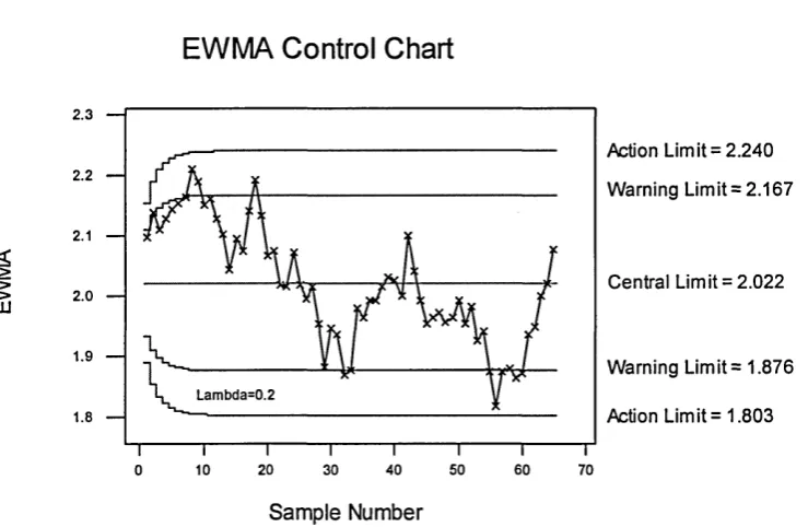
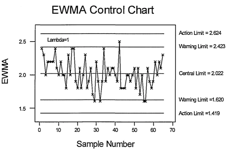
Optimum design criteria for EWMA control chart can be found from Crowder (1987) and Lucus and Saccucci (1990) who derive theoretical properties for the chart in order to ARL. The latter compare EWMA chart to the CUSUM chart, concluding that there is little difference between them.

2.8 Multivariate Control Chart

Control charts play a very important role in industrial situations for monitoring processes. Multivariate control chart is necessary when monitoring of several correlated quality characteristics simultaneously is desired. Traditional multivariate control chart based on f 2 statistics, which are very effective for detecting events, when the multivariate space is not very large, (Kourti and MacGregor, 1996).

Many of the concepts of multivariate quality control are associated with Hotelling (1947). Several approaches to multivariate control chart have been discussed in the literature such as economic design, can be found in Alt (1985), chart based on principle components can be found in Jackson (1980,1981a, 1981b, 1985), Ryan (1989) and Montgomery (1997). Jackson (1985) proposed using principle component analysis (PCA) for selecting the problem variables. The PCA technique decomposes the

j 1 statistic into a sum of independent squared principal components, which are linear combinations of the original variables. These principle components must be examined to see why the process is statistical out of control.

Alloway (1994) have considered the accuracy of multivariate control charts. The latter can be improved through a three step graphic process: identify and remove outliers, examine the distribution of the data relative to assumptions and use alternative approaches if the assumption of normality is not justified.

The values plotted on multivariate control charts are usually statistical based on his well-known Hotelling’s f 2 distribution. This distribution is the multivariate counterpart to student's t distribution. The multivariate j 2 chart is particularly appropriate when the characteristics of interest are correlated.

In constructing the multivariate control charts, it is assumed that the covariance matrix is constant over time. One of the visual method for checking this assumption is to monitor the process variability.

An obvious idea is to consult the corresponding univariate control charts when a multivariate control chart signals that the process is out of control. Two aspects must be considered. Firstly, the overall significance level of the simultaneous use of p univariate control charts is difficult to determine. Secondly, it is not necessarily one quality characteristic that causes an out of control situation.

Development of Multivariate Control Chart

The SPC approach for process monitoring, currently in practice in several industries, is to chart a small number of variables, usually the final product quality variables, and examine them one at a time. However, when the quality of a product is defined by more than one property, all the properties should be studied collectively. Multivariate SPC charts developed for this purpose have been based on the %2 statistics or on Hotelling

jr2 statistic.

x 2

= O- Ao)' Xo

Where % denoted the (Px 1) vector of sample mean and %2ap is corresponding

j 2 -percentile. Plotting the value of %2 versus time with an upper control limit (UCL) given by %2atP, where a is an appropriate significance level for performing the test (e.g. a = 0.05 or 0.01). The %2 statistic represents the direct or weighted distance (Mahalanobis distance) of any point from ^ . If ^ 2 statistic plot above the upper control limit, the process mean is out-of-control, and assignable causes of variation are sought. For the two quality characteristics, an elliptical control region, centred at ^ , can be used in place for %2 -chart.

When the in-control covariance matrix £ is not known and must be estimated from a limited amount of data, it is suitable to plot Hotelling f 2 statistic given by

T 2 = (x - x)' s '1 (x - x)

Where s is an estimate of covariance matrix £ . An upper control limit t2cl is then obtained based on the F distribution and will depend upon the degree of freedom available for the estimate s, (Wierda, 1994a).

The phase 1 control limits for the p 2is given by

_ p(m -l)Q i-l)

U L / L — _{m n - m - p + 1}, , r a , p , m n - m - p+ 1

LCL = 0

chart is used for monitoring future production, the control limits

r p(m + l)(n -1) ^

. r a ,p ,m n - m - p+ 1

m n - m - p + 1

LCL = 0

where 77 is Snedecor's F with y and y degree freedom, p is the number of quality_{Vi ,V2 1 2} characteristics , m is number of preliminary sample and n is size of preliminary sample.

When n and £ are estimated from a large number of preliminary samples, it is customary to use UCL=^2ap as the upper control limit in both phase 1 and phase 2. Retrospective analysis of the preliminary samples to test for statistical control and establish control limits also occurs in the univariate control chart setting. For the j - chart, it is well known that if we use m >20or 25 preliminary samples, the distinction between phase 1 and phase 2 limits will nearly coincide, (Montgomery, 1997, pp: 366- 367).

Multivariate control chart for individual case i.e. n=l

This case always occurs in the chemical and process industries. Since these industries frequently have multiple quality characteristics that must be monitored, multivariate control charts with n=l.

Suppose that m sample (preliminary sample), each of size n=l are available, and that p is the number of quality characteristics observed in each sample. Let x and s be the sample mean vector and covariance matrix, respectively, of these observations. The Hotelling p 2 statistic in the above becomes

T 2 = ( x - x)'s~l (x - x)

p 2 test statistic is distributed as

T * _ p ( p / 2 , ( m - p -1) /2)

m

see Sullivan and Woodall (1996) and Gnanadesikan and Kettenring (1972).

Then the control limits for this statistic are suggested by Tracy ef ai (1992) as follows

UCL = *j3(a/2; p / 2 , ( m - p - 1)/2)

m

( m -1) 2 ( p / ( m - p - \ ) F ( a l 2 \ p , m - p - l )

m I + (p /(m — p — I)) F ( a / 2; p , m — p — V)

and

LCL = & L J L * p ( i _ a /2; p / 2 , ( m - p - 1)/2)

m

_ (in - 1) 2 ^ (p /{pi - p - 1) F { 1 - a ! 2; p , m - p - Y )

m \ + ( p / ( m - p p , m - p - I )

where 0 ( a / 2 ; p / 2 , ( m - p —1) /2) and j 3 ( \ - a / 2 ; p / 2 , ( m - p - l ) /2)are.the 1 _ ££ percentile of the beta distribution.

As well as control limits for a single^/ multivariate observation vector and an estimate s based on m past multivariate are

rim _ + „

m — mp LCL = 0

and when the number of preliminary sample is large, i.e. m>1 0 0, many practitioners use an approximate control limit

2.9 Mixture distribution

Mixture distribution needs when the data represented by two or more kinds of distribution, for example, Laplace and Normal distribution. In this thesis the author assumes that the data from the mixture distributions are statistically independent from each other.

Statistical analysis of mixture data has proved not to be straightforward, for two main reason. Firstly, explicitly formulae generally do not exist for estimators of the various parameters, so the numerical methods are required. Secondly, theoretical difficulties which arise in certain aspects of the statistical analysis reveal some common mixture problems to be non-standard .

As a result, detailed investigation of the analysis of finite mixture problems offers more than just a catalogue of straightforward applications of standard methods to a particular class of statistical methods.

In this thesis will dealing with quantile approach for mixture distribution in order to develop quality control chart.

2.10 Effect o f Non-normality on control chart

One of the underlying assumptions of SPC is the use of the normal distribution. Such assumptions are implicit in the construction of control charts and process capability studies. It has long been realised that the variability associated with many engineering processes does not have a normal distribution. In continuous batch manufacture the normality assumption is often justified, but the distribution of the process variation is more critical when considering the sample sizes associated with small batch manufacture.

these cases a transformation would be inappropriate. It is thus that the data be taken from a stable process.

Schilling and Nelson (1976) investigated the effect of non-normality on charts and concluded that the non-normality is usually not a problem for subgroup sizes of four or more. For smaller subgroup sizes, and especially for individual measurements, non­ normality can be serious problem.

Control charts and process capability calculations remain fundamental techniques for statistical process control. However, it has long been realised that the accuracy of these calculations can be significantly affected when sampling from a non-normal population. Many quality practitioners are conscious of these problems but are not aware of the effects; such problems might have on the integrity of their results. Use is made of the Johnson system of distributions as a simulation technique to investigate the effects of non-normality of control charts and process control calculations. An alternative technique is suggested for process capability calculations which alleviates the problems of non-normality while retaining computational efficiency, (Spedding, 1994).

In general, there is the need for widespread realisation that non-normality can be a major problem for a wide variety of control chart procedures. For sample sizes, less than five, the central limit theorem does not apply. This has been demonstrated for an

X chart by Yourstone and Zimmer (1992), Ryan and Howley (1999), Janacek and

Meikle (1997) , Moore (1957) and for attributes charts by Ryan and Schwertman (1997) and Ryan (1989).

For positively skewed data, simple transformations such as the logarithmic, cube root or square are often useful. If we are dealing with proportions and if binomial variations is found, the inverse sine of the square root may remedy the problem.

interpretation of control charts. In such circumstances, the standard method of assuming a normal distribution may perform poorly, especially for very skewed process distribution, (Burr, 1967) and (Schilling & Nelson, 1976).

The above literature review indicates that there are real problems in dealing with statistical process control for non-normal distributions and mixture distributions. The main purpose of this thesis is to develop quality control charts and capability index for non-normal distribution and mixture distribution which can be easily adopted by the practitioner of statistical process control.

Chapter 3: Control Chart Methodology for

Non-Normal Situation

3.1 Introduction

In general, Shewhart control charts assume that the set of data comes out from the process, following normal distribution, and the probabilities of points falling outside control limits, when the process is in control is 0.0027. Hence, most of SPC techniques have been derived and constructed from the concept of quality characteristics which depends on normal distribution, (see the reference of the central limit theorem in chapter 2). In reality, often the set of data such as, chemical process data, lifetimes data and cutting tool wear processes are not normal. So when constructed, a control chart of * or r , supposes that the data is normal and the actual sets of data are not normal. Therefore, it will give inaccurate results of quality characteristics.

There are some useful and validity techniques for transforming the non-normal data to normality situation. Therefore, it is possible to perform SPC technique on non-normal data. Rigdon, et al. (1994) suggest two remedies for dealing with non-normality, using a suitable non-normal distribution for a particular data, by physical consideration of the process; and seeking a transformation of the original data, which leads to an approximate normal distribution. From the literature search, it was found that there are many techniques used for such procedures. This chapter deals with some of these techniques, such as Quesenberry transformation or Q-Chart, Box-Cox transformation (1964) and Quantile Approach. In addition, there are other techniques, such as Johnson transformation, Pearson System and others, which will not be discussed here.

3.2 Quesenberry Technique (Q-Chart)

Statistical Transformation

In classical mathematics e.g. Laplace transformation when the original data is transform and a solution is found we perform an iverse transformation on the situation. Thus the solution refers to the original data. However, in statistics when we perform a transformation we model the relationships and solution in the transformation space only and by inference we claim that the same relationship exist in the original data. Quantile technique overcome this deficiency of refered to the original data at all times.

Quesenberry (1991) has suggested a new technique for short-run SPC using a transformation. This technique plays a role in monitoring a process mean or variance for a normally distributed quality variable. He refers to this technique as Q-Chart and defines it as being distributed approximately as standard normal statistics and is also approximately independent. The technique is plotted on standard normal scale, when the parameters are known and unknown. He notes that, the technique can be used for short- run and for long-run production

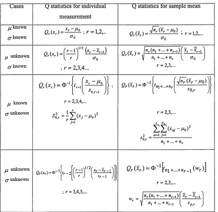
Quesenberry uses the Q-chart for variable data x,s or R and for individual measurement of the process mean and the process variance. Both processes are discussed for the four cases below, which are, (^ known, a known); ( ^ unknown, G known); known,

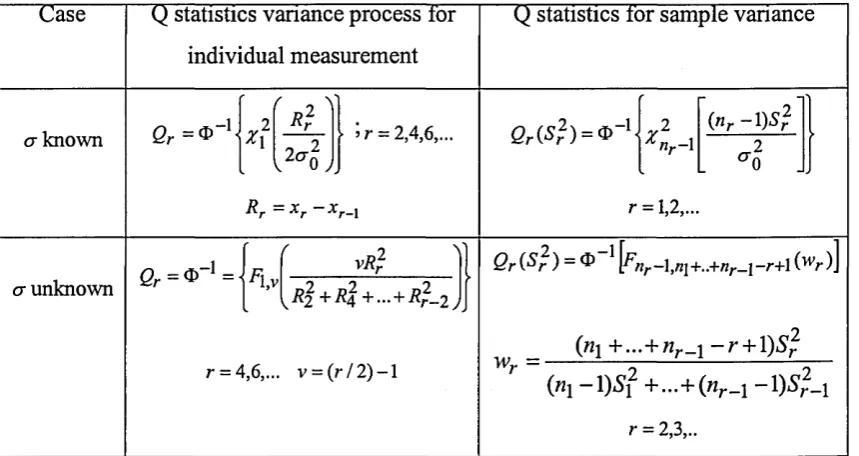
Q- unknown) and unknown, a unknown). Table 1 provides the Q statistics for individual measurement and Q statistics for sample mean, and Table 2 provides the Q statistics variance process for individual measurement and Q statistics for sample variance.

Table 1: Quesenberry statistics from sample mean

Q statistics tor individual measurement

Q statistics for sample mean Cases

jU known

(j known Q r ( x r ) = ^ — ^ - - , r = 1 , 2 , Q r ( x r ) = - > r = 1,2,...

j unknown ( j known

Q r (x r) = ( x r - x r_i) Q r ( Xr ) =

CTn

n r ( n x + . . . + n r _l )

; r = 2,3,4...

«! + ... + n r r = 2,3,...

f - - ^

x r ~ Xr- 1

k °o ;

j j known

( j unknown

-l r / \

' * r 1

0

1

H

>

{ S 0,r-l )

-1

Qr(xr ) ~ ® yn\+...+nr yjnr Cxr MO ) s 0,r

r = 2,3,4,...

Slr

r j=1

r = 2,3,... r na

2 _ g»i M

s 0,r ~

unknown _{Qr(xr) = O X\tr-2} (j unknown

r - 1 j xr -x r -\

r J I sr-l

Q r ( x r ) ~ ® \ n \n \ + . . . + n r . +...+/Jr_j C^V)] r = 2,3,...

;r = 3,4,5,...

n r ( n x + . . . + n r _ l )

«! + ... + nr_j

Table 2: Quesenberry statistics from sample variance Case Q statistics variance process for

individual measurement

Q statistics tor sample variance

a known e r = ® " ‘-V

*r'-Rr '

= xr - x

► ’ r = 2,4,6,...

r - 1

Q A S ? ) = ©

-1-r x l - i

= 1,2,...

(»r - W ?

[ J

>

a unknown e r = 4 .-| = |f i iV_{[ F-2 + R%}vRr _{+... + R}-2 Jj}j| Qr (Rr ) - ^ j/7nr +..+«r_j -r+\ (wr )] (Wj + ... + T27._j — V + 1)jS'^ r = 4,6,... v = ( r /2 )-l

(»! -1)5? +...+ («r_!-1)^2_! r = 2,3,..

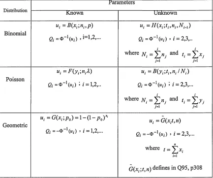
Quesenberry also applies the Q-chart for attributes of Binomial, Poisson and Geometric distributions. Q-chart can be applied for common distribution, which are used to describe variable and attribute data. Table 3 gives the summary of Q-chart for attributes of such distributions. The transform observations from such distributions are given in table 3, for attribute case, values plotted on standardised normal Q charts, for the two cases when the parameter is known and unknown before charting is begun.

By transforming the observations through such distributions function in the table 3, the

u 's are approximately uniform on (0,1), and the q_'s are approximately standard

Table 3: Quesenberry statistics for attribute

Distribution _Known Parameters _Unknown

Binomial

Uj = B{x,',n,,p)

Qi =4>_1(»,)

ut =H(x,;t„nl,Nl_l)

Qi =4>_1(«,) , i= 2,3,..

where N , = £ « . and ti = £ *

,-j .i j - t

Poisson

ut =F(y,\ntX)

Qi = « “'(«/) ; / = 1,2,..

u, =B(yi\t„nl IN l)

Qi=9~\ui) ; / = 2,3,...

where N . = and t . = ^ y .

7=1 7=1

Geometric

u, =G(x,;p0) = ! - ( } - p 0)x‘

Qi=-®-'(ui) > i = 1.2....

u{ = G{xiti n)

e/= -® _1(«,-) > i =2,3,...

where / = £ * . i=1

G(x.;t,n) defines in Q95, p308

Quesenberry concludes from the distributions above, that Q-chart can be applied for these two cases. The interpretation of the Q-charts for the two cases, are nearly the same, but basic differences must be borne in mind. Q-chart for unknown parameters are plotted from the second sample, but no points are plotted for the first sample because, the parameter must be estimated from the set of data. Meanwhile, Q-chart for known parameters are plotted from the first sample. Quesenberry discussed some examples where to apply Q-chart on the distributions above. The observations plotted on these charts were very similar for both cases, when parameters are known and unknown.

the 1-of-l test, have poor sensitivity. Whereas, the test consisting of four out of five points beyond one sigma control limits i.e. the 4-of-5 test, is found to be a good test. The EWMA and CUSUM Q charts are most sensitive and are nearly comparable in overall performance.

Del Castilo and Montgomery (1994) have investigated the average run length performance of the Q-chart for variables and show that in some cases the ARL performance is inadequate. They suggested some modifications to the Q-chart procedures and some alternative methods based on the EWMA and a related technique called the Kalman filter which have better ARL performance than the Q-chart.

3.3 Box-Cox Transformation

Most statistical methods were created under the assumption of normality. Shewhart (1931) mentioned that most industrial measurements violate this assumption. Quality characteristics are always required to be normally distributed. If quality characteristics are not normally distributed, but the techniques are based on normality, then we will have inaccurate results. So, it is important to transform the data to normal situation. In most cases, the choice of the transformation is not obvious. For positive measurements, i.e. skew to the right, a family of power distribution was introduced by Tukey (1957). It is convenient to transform the data to normality using the formula below

yt =xf ;A * 0

yj = log*. ;A = 0

One of the best techniques for choosing a transformation which could simultaneously achieve:

1- normality of distribution

is Box and Cox's (1964). In addition, such transformation chosen to achieve independence between cell mean and cell variance often has the effect of improving the closeness to normality.

Box and Cox suggested a useful modification for family of power transformation, which is defined only for positive values, using a maximum likelihood estimate of

x-However, this technique is not a restrictive one, because a single constant can be added to the data if there are some negative values.

y w =y\ogy ;A = 0

Where y = (]!"_, y.)lln = exp(-Zlnyf) ;y. >0 is the geometric mean.

n

The family of power transformations are chosen, where each value is replaced by x* at where x always one of the value below:

X -2 -1 -0.5 0 0.5 i 2

^

—

H

II 1 1

xl

1

*,°'5

log*,

For x =-0.5 ,0 ,0.5, the data values must all be positive. To use these transformations when there are negative and positive values, a constant can be added to all the data values, which must be greater than 0. If all the data values are negative, the data instead should be multiplied -1. However, in this situation, data suggesting skewness to the right would now become data suggesting skewness to the left.

3.4 New Approach

Quantile function Q(p) can be used to provide non-parametric measures of location, scale etc. Q(p) can be applied for continuous and discrete random variable. Unfortunately, Q(p) does not exist for all points of the p thquantile in case of discrete random variable, but it gives general indication on the attitude of set of data. Q(p) is defined as the inverse of distribution function of the random variable. So quantile function is defined as Q(p) = F~1(p), 0 <p <l > the sample quantile function define as

Q(p) = f- \p) =x, < P <

-n n

The density quantile function f(Q(p)) can be obtained by deriving the quantile distribution function

P = F(Q(P)) 3.1

where and q q are the inverse function of each other.

Differentiation (3.1) in respect to p

1 = f(x)q(j>) ; x = Q(p)

then

f(x) = \lq(p)

is the density quantile function. So a plot yy*) against x = Q(p), will give the desired density plot. For more details see Parzen 1979.

Quantile population q for standard normal distribution N(0,1) are defined by

P ( X < %)) = Pu)= f -n + l

If the data follows a normal distribution, the plotting of theoretical quantile against observed quantile will be approximately linearly related. If the plotting of data does not give linear, then the derivation from this line will reveal how the distribution differs. So, the quantile approach for non-normal situation is discussed here.

For non-normal distribution, data can be transformed to normality, by using the square root for all random variable, Somerville and Montgomery (1996) or by taking the fourth root of the data, Kittlitz (1999). Moreover, some authors have recommended the use of distribution of power family or its extension, as done by Box-Cox (1964). On the other hand, Quesenberry technique (1991) can be used for common distribution, in order to deal with non-normal data.

The advantage of the quantile method is that it is very simple and fully applicable and can be easily used by a practitioner. Quantile approach also plays a very important role in continuous random variable.

Chapter 4: Theoretical Development of Quantile

Approach

4.1 Introduction

Statistical process control techniques are widely used in industry for process monitoring and quality improvement. Various statistical control charts have been developed to monitor the process mean and variance. Traditional SPC methodology is based on the fundamental assumption that the process data are statistical normal distributed. Although, the process data are always non-normal distributed, (see Box and Luceno, 1997, p.6). For example, Chemical reactions follow Logistic; Bulb life follow Weibull, Power, Lognormal; Mechanical properties of material follow Extreme-value, etc.

As discuss before, the effects of non-normality on quality control charts have been suggested by Schiling and Nelson (1976), and concluded that the non-normality is usually not a problem for subgroup size of four or more. But for small subgroup size and especially for individual measurements, non-normality can be a serious problem. There are two ways of dealing with non-normality: firstly, using an appropriate non­ normal distribution for the particular data suggested by the physical considerations of the process charts for the Weibull distribution (see Nelson, 1979) and secondly, seeking a transformation of the original data that results in an approximate normal data, such as the Box-Cox transformation, SPC Q chart proposed by Quesenberry, (1995) and the use of distribution families, e.g. Pearson, Johnson.

data, it is sometimes difficult for people to interpret the various approaches of statistical process control, especially when they are modified with the help of various transformations (DuBois ei ai 1991).

It is desirable that the data for statistical control charts be normally distributed. However, if the data is not normal, then a transformation can be used to produce a suitable control chart. A control chart is proposed which monitors the conformance of a sample using the quantile or inverse cumulative distribution function. This method also helps to detect changes in the distributional shape, which may be undetected in control charts that are based on summary statistics.

A successful quality improvement process must be based on proper interpretation of statistical data and quality improvement methods. In this chapter we will be discussing quality improvement process through quantile distribution. In doing so we will first discuss the quantile process of monitoring and control, then develop a quality control chart for this purpose using the median rankit.

4.2 Quantile Approach

Tukey (1960) has introduced a family of random variables defined by the transformation

xf = [ p x - ^ - p f V X 4.1

where p is a uniformly distributed random variable on (0,1) and — oo -< /L -< oo • It can be shown that the rectangular and logistic distributions are also members of the above family. For example a limiting form of (4.1) when ^ Q is given by

where x is known as the quantile function o f logistic distribution. Location and scale parameters could be introduced to obtain the Generalised Lambda Distribution (GLD), which is also true for all quantile distribution function. One of the important aspects of the lambda family is that the percentage points are available directly for use (Joiner & Rosenblatt, 1971).

Various distributions about Generalised Lambda Distributions (GLD) can be found in Shapiro & Gross (1981), Ramberg and Schmeiser (1972) and Ramberg & ai (1979). However, a new quantile distribution can be obtained by using the inverse function of the generalised lambda distribution. For example, in GLD, a new quantile distribution, which is an extension of Tukey lambda distribution, Ramberg and Schmeiser (1974), can be obtained as follows

~ { \ - p ) l'}IX2 - , Q < P < 1 4.3

where the range of r can be determined by setting p=0 and p= l. Range of x values

p

are discussed in Ramberg (1974), e.g. if X2, A, and ^ a re all-negative and x 2 -» 0 then the range is

(_oo,oo)-In equation (4.3), if p is a uniform random variable, then x will have a GLD. The skewness and peakedness of the GLD can be determined by ^ and x4 and. the scale by

X2. The location of GLD can then be given any value using appropriate choice of xi • However, if the GLD is asymmetric (x3 ^ X4)> then its expected value will not be equal to xi as is the case with the symmetric situation. Furthermore, if x3 =A4> the original lambda distribution will be given, i.e. symmetric random variable.

Suppose x be a random variable with a distribution function F. The root of equation

F(xp) = P = prob(X < xp)

is called the p-th quantile of the distribution F(xp) • The p-th quantile is also called the lOOpth percentile. The p.-th percentile of the population described by the distribution Q(p) is simply Q(pt)> where lOO/?,-^ is a suitable percentage. The root of the above equation, for p=0.5, is corresponds to the median of F, and for p=0.25 and p=0.75 which correspond to the lower and upper quantiles of F.

Here, the inverse cumulative distribution or quantile distribution Q (p) can be expressed as follows

= Q(P) = F~\p) = [x : F(x) = p i p e (0,1)

Here, F (x), f (x) and Q (p) (i.e. cumulative distribution, density function and quantile distribution, respectively) can be used as alternative starting points for defining distributions (Parzen, 1979). Quantile density function is defined as

/(GOO) = i/*Q 0

Kanji & Arif (2000) have shown that the quantile approach can be used to develop the quantile distribution, which can be used to develop a control chart. For example, if we consider a distribution with parameters X^rpQ where q represents one or more

parameters, e.g. Weibull, Pareto, Power, then Q(p) is

Q(p) = ^ + tjR(p; 0) 4.4

can be defined as a quantile distribution. A standard quantile distribution can be expressed as

x - X

= R(P,0) n

Furthermore, a quantile distribution, which requires only two parameters (i.e. location and scale parameters), can be expressed as

Q(,P) = A + t}R(p) 4.5

where R(p) does not depend on the parameter (#). Distributions such as Exponential, Extreme value and Uniform belong to this category.

Probability rules for Quantile Approach

Various pro