Excel 2013
Excel 2013: The Missing Manual
by Matthew MacDonaldCopyright © 2013 Matthew MacDonald. All rights reserved. Printed in the United States of America.
Published by O’Reilly Media, Inc.,
1005 Gravenstein Highway North, Sebastopol, CA 95472.
O’Reilly books may be purchased for educational, business, or sales promotional use. Online editions are also available for most titles (http://my.safaribooksonline.com). For more information, contact our corporate/institutional sales department: (800) 998-9938 or [email protected].
April 2013: First Edition.
Revision History for the Nth Edition: 2013-04-10 First release
See http://oreilly.com/catalog/errata.csp?isbn=9781449357276 for release details.
The Missing Manual is a registered trademark of O’Reilly Media, Inc. The Missing Manual logo, and “The book that should have been in the box” are trademarks of O’Reilly Media, Inc. Many of the designations used by manufacturers and sellers to distinguish their products are claimed as trademarks. Where those designations appear in this book, and O’Reilly Media is aware of a trademark claim, the designations are capitalized.
Contents
The Missing Credits
. . .ix
Introduction
. . . .xiii
Part One:
Worksheet Basics
CHAPTER 1:Creating Your First Spreadsheet
. . .3
Starting a Workbook . . . 3
Adding Information to a Worksheet . . . 4
Using the Ribbon . . . 12
Using the Status Bar. . . 19
Going Backstage . . . 23
Saving Files . . . .26
Opening Files. . . 41
CHAPTER 2:
Adding Information to Worksheets
. . .47
Adding Different Types of Data . . . 47
Handy Timesavers . . . .56
Dealing with Change: Undo, Redo, and AutoRecover . . . .69
Spell-Check . . . 75
Adding Hyperlinks . . . .80
CHAPTER 3:
Moving Data
. . .85
Selecting Cells . . . .85
Moving Cells Around . . . .92
Adding and Moving Columns or Rows . . . 103
CHAPTER 4:
Managing Worksheets
. . .107
Worksheets and Workbooks . . . 108
Find and Replace . . . 118
CHAPTER 5:
Formatting Cells
. . .127
Formatting Cell Values . . . 128
CHAPTER 6:
Smart Formatting Tricks
. . .165
The Format Painter. . . 165
Styles and Themes . . . 166
Conditional Formatting . . . 179
CHAPTER 7:
Viewing and Printing Worksheets
. . .189
Controlling Your View . . . 189
Printing . . . .202
Controlling Pagination . . . 214
Part two:
Formulas and Functions
CHAPTER 8:Building Basic Formulas
. . .221
Creating a Basic Formula . . . 221
Functions . . . .227
Formula Errors . . . .234
Logical Operators . . . .238
Formula Shortcuts . . . 240
Copying Formulas . . . .248
CHAPTER 9:
Math and Statistical Functions
. . .261
Rounding Numbers . . . 261
Groups of Numbers . . . .267
General Math Functions . . . .279
Trigonometry and Advanced Math . . . .288
Advanced Statistics . . . .292
CHAPTER 10:
Financial Functions
. . .297
The World of Finance . . . .297
Financial Functions. . . .298
Depreciation . . . 312
Other Financial Functions . . . 315
CHAPTER 11:
Manipulating Dates, Times, and Text
. . .319
Manipulating Text . . . 319
Manipulating Dates and Times . . . .328
CHAPTER 13:
Advanced Formula Writing and Troubleshooting
. . .375
Conditions in Formulas . . . .375
Descriptive Names for Cell References . . . 384
Variable Data Tables . . . .395
Controlling Recalculation . . . 400
Solving Formula Errors . . . 401
Part three:
Organizing Your information
CHAPTER 14:Tables: List Management Made Easy
. . .413
The Basics of Tables . . . 414
Sorting a Table . . . .424
Filtering a Table. . . 430
Dealing with Duplicate Rows . . . .436
Performing Table Calculations . . . .438
CHAPTER 15:
Grouping and Outlining Data
. . .451
Basic Data Grouping . . . .452
Grouping Timesavers . . . 464
CHAPTER 16:
Templates
. . . .469
Using the Office Online Templates . . . .470
Rolling Your Own Templates . . . .479
Part Four:
Charts and Graphics
CHAPTER 17:Creating Basic Charts
. . . .487
Charting 101 . . . 488
Basic Tasks with Charts . . . .495
Practical Charting . . . .502
Chart Types . . . 512
CHAPTER 18:
Formatting and Perfecting Charts
. . .527
Chart Styles and Layouts . . . .527
Adding Chart Elements . . . 531
Formatting Chart Elements . . . .543
Improving Your Charts . . . .556
Advanced Charting . . . .568
CHAPTER 19:
Inserting Graphics
. . .577
Adding Pictures to a Worksheet . . . .578
Excel’s Clip Art Library . . . .593
Drawing Shapes . . . .596
CHAPTER 20:
Visualizing Your Data
. . . .611
Data Bars . . . 612
Color Scales . . . .622
Icon Sets . . . .623
Sparklines . . . .627
Part Five:
Sharing Data with the Rest of the World
CHAPTER 21:Protecting Your Workbooks
. . .639
Understanding Excel’s Safeguards . . . .639
Data Validation . . . 640
Locked and Hidden Cells . . . .652
CHAPTER 22:
Worksheet Collaboration
. . . .663
Your Excel Identity . . . 664
Preparing Your Workbook . . . .665
Distributing Your Workbook . . . 671
Adding Comments . . . .674
Tracking Changes . . . .679
Sharing Your Workbook . . . 690
Reviewing Workbooks with Inquire . . . 696
CHAPTER 23:
Using Excel on the Web
. . .705
Putting Your Files Online. . . .705
Using the Excel Web App . . . 714
Sharing Your Files . . . .724
CHAPTER 24:
Exchanging Data with Other Programs
. . .739
Sharing Information in Windows . . . .740
Embedding and Linking Objects . . . 741
Transferring Data . . . 751
Part six:
Advanced Data Analysis
CHAPTER 25:Scenarios and Goal Seeking
. . .763
Using Scenarios . . . .764
Using Goal Seek . . . 771
CHAPTER 26:
Pivot Tables
. . .791
Summary Tables Revisited . . . .792
Building Pivot Tables . . . .795
Multi-Layered Pivot Tables . . . 806
Fine-Tuning Pivot Table Calculations . . . 811
Filtering a Pivot Table . . . 815
Pivot Charts . . . .826
CHAPTER 27:
Analyzing Databases
. . .831
Excel and Databases . . . 831
Creating a Data Connection . . . .833
The Data Model: Boosting Pivot Tables . . . 846
CHAPTER 28:
Analyzing XML and Web Data
. . .861
Understanding XML . . . .862
Retrieving Information from XML . . . .867
Creating Web Queries . . . .879
Connecting to Online Data Services with OData . . . .883
Part seven:
Programming Excel
CHAPTER 29:Automating Tasks with Macros
. . . .893
Macros 101 . . . .893
The Macro Recorder . . . 896
Macro Security . . . 903
Creating Practical Macros . . . 911
CHAPTER 30:
Programming Spreadsheets with VBA
. . .919
The Visual Basic Editor . . . 920
Understanding Macro Code . . . .926
Exploring the VBA Language . . . 930
Part eight:
Appendix
APPENDIX A:Customizing the Ribbon
. . . .945
Adding Your Favorites to the QAT . . . 946
Personalizing the Ribbon . . . 951
The Missing Credits
ABOuT ThE AuThOR
Matthew MacDonald (author) is a four-time Microsoft MVP and a technology writer with well over a dozen books to his name. Office geeks can follow him into the world of databases with
Access 2013: The Missing Manual. Web fans can build an online home with him in Creating a Website: The Missing Manual. And human beings of all description can discover just how strange they really are in the quirky handbooks Your Brain: The Missing Manual and Your Body: The Missing Manual.
ABOuT ThE CREATivE TEAM
Peter McKie (editor) graduated from Boston University’s School of Journalism and lives in New York City. In his spare time, he manages the Facebook page and website that chronicle the history of his summer community. Email: [email protected]. Melanie Yarbrough (production editor) lives and works in Cambridge, MA. When not ushering books through production, she’s sewing, writing, and baking whatever she can think up. Email: [email protected].
Julie Hawks (indexer) is an indexer for the Missing Manual series. She is currently pursuing a master’s degree in Religious Studies while discovering the joys of warm winters in the Carolinas. Email: [email protected].
Carla Spoon (proofreader) is a freelance writer and copy editor. An avid runner, she works and feeds her tech gadget addiction from her home office in the shadow of Mount Rainier. Email: [email protected]
.
Zack Barresse (technical reviewer)is a Microsoft Excel MVP and has held that title for seven consecutive years. He works as a full-time firefighter in his hometown of Boardman, Oregon, where he resides with his wife and four children.
ACknOWlEDGMEnTS
Writing a book about a program as sprawling and complex as Excel is a labor of love (love of pain, that is). I’m deeply indebted to a whole host of people who helped out with this edition and the three previous ones. They include Peter McKie, Nellie McKesson, Brian Sawyer, Peter Meyers, Sarah Milstein, and technical reviewers Zack Barresse, and Stephanie Dukes. I also owe thanks to many people who worked to get this book formatted, indexed, and printed—you can meet many of them in the section “About the Creative Team,” above.
Completing this book required a few sleepless nights (and many sleep-deprived days). I extend my love and thanks to my daughters Maya and Brenna, who put up with it without crying most of the time, my dear wife Faria, who mostly did the same, and our moms and dads (Nora, Razia, Paul, and Hamid), who contributed hours of babysitting, tasty meals, and general help around the house that kept this book on track. So thanks everyone—without you half of the book would still be trapped inside my brain!
—Matthew MacDonald
ThE MiSSinG MAnuAl SERiES
Missing Manuals are witty, superbly written guides to computer products that don’t come with printed manuals (which is just about all of them). Each book features a handcrafted index and cross-references to specific pages (not just chapters). Recent and upcoming titles include:
• Access 2010: The Missing Manual by Matthew MacDonald • Access 2013: The Missing Manual by Matthew MacDonald • Adobe Edge Animate: The Missing Manual by Chris Grover • Buying a Home: The Missing Manual by Nancy Conner
• Creating a Website: The Missing Manual, Third Edition by Matthew MacDonald • CSS3: The Missing Manual by David Sawyer McFarland
• David Pogue’s Digital Photography: The Missing Manual by David Pogue • Dreamweaver CS6: The Missing Manual by David Sawyer McFarland • Droid 2: The Missing Manual by Preston Gralla
• Droid X2: The Missing Manual by Preston Gralla
• Galaxy Tab: The Missing Manual by Preston Gralla • Google+: The Missing Manual by Kevin Purdy • HTML5: The Missing Manual by Matthew MacDonald
• iMovie ’11 & iDVD: The Missing Manual by David Pogue and Aaron Miller • iPad: The Missing Manual, Fifth Edition by J.D. Biersdorfer
• iPhone: The Missing Manual, Fifth Edition by David Pogue
• iPhone App Development: The Missing Manual by Craig Hockenberry • iPhoto ’11: The Missing Manual by David Pogue and Lesa Snider
• iPod: The Missing Manual, Tenth Edition by J.D. Biersdorfer and David Pogue • JavaScript & jQuery: The Missing Manual, Second Edition by David Sawyer
McFarland
• Kindle Fire HD: The Missing Manual by Peter Meyers • Living Green: The Missing Manual by Nancy Conner • Mac OS X Lion: The Missing Manual by David Pogue
• Microsoft Project 2010: The Missing Manual by Bonnie Biafore • Microsoft Project 2013: The Missing Manual by Bonnie Biafore • Motorola Xoom: The Missing Manual by Preston Gralla • Netbooks: The Missing Manual by J.D. Biersdorfer • NOOK HD: The Missing Manual by Preston Gralla
• Office 2010: The Missing Manual by Nancy Conner and Matthew MacDonald • Office 2011 for Macintosh: The Missing Manual by Chris Grover
• Office 2013: The Missing Manual by Nancy Conner and Matthew MacDonald • OS X Mountain Lion: The Missing Manual by David Pogue
• Personal Investing: The Missing Manual by Bonnie Biafore • Photoshop CS6: The Missing Manual by Lesa Snider
• Photoshop Elements 11: The Missing Manual by Barbara Brundage • PHP & MySQL: The Missing Manual, Second Edition by Brett McLaughlin • QuickBooks 2012: The Missing Manual by Bonnie Biafore
• QuickBooks 2013: The Missing Manual by Bonnie Biafore
• Windows 7: The Missing Manual by David Pogue • Windows 8: The Missing Manual by David Pogue • WordPress: The Missing Manual by Matthew MacDonald • Your Body: The Missing Manual by Matthew MacDonald • Your Brain: The Missing Manual by Matthew MacDonald • Your Money: The Missing Manual by J.D. Roth
M
ost people don’t need much convincing to use Excel, perhaps the world’s premier spreadsheet software. Its overwhelming popularity, especially in the business world, makes it the obvious choice for millions of number crunchers. But despite its wide use, few people know where to find Excel’s most impressive features or why they’d want to use them in the first place. Excel 2013: The Missing Manual fills that void, explaining everything from basic Excel concepts to the fancy tricks of the trade.This book teaches you how Excel works, and shows you how to use Excel’s tools to answer real-world questions like “How many workdays are there between today and my vacation?”, “How much money do I need in the bank right now to retire a millionaire?”, and “Statistically speaking, who’s smarter—Democrats or Republicans?” Best of all, you’ll steer clear of obscure options that aren’t worth the trouble to learn, while homing in on the hidden gems that will win you the undying adoration of your coworkers, your family, and your friends—or at least your accountant.
What You Can Do with Excel
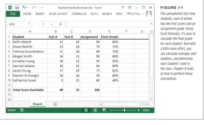
Excel and Word are the two powerhouses of the Microsoft Office family. While Word lets you create and edit documents, Excel specializes in letting you create, edit, and analyze data that’s organized into lists or tables. This grid-like arrangement of information is called a spreadsheet. Figure I-1 shows an example.
WhaT You Can Do WiTh
[image:16.504.36.445.91.341.2]ExCEl
FiGuRE i-1
This spreadsheet lists nine students, each of whom has two test scores and an assignment grade. Using Excel formulas, it’s easy to calculate the final grade for each student. And with a little more effort, you can calculate averages and medians, and determine each student’s rank in the class. Chapter 8 looks at how to perform these calculations.
NOTE Excel shines when it comes to numerical data, but the program doesn’t limit you to calculations. While it has the computing muscle to analyze stacks of numbers, it’s equally useful for keeping track of the Blu-rays in your personal movie collection.
Some common types of spreadsheet include:
• Business documents like financial statements, invoices, expense reports, and earnings statements.
• Personal documents like weekly budgets, catalogs of your Star Wars action figures, exercise logs, and shopping lists.
WhaT You Can Do WiTh
ExCEl
predictions for the future. Excel can help track your investments and tell you how long until you’ll have saved enough to buy that weekend house in Vegas.
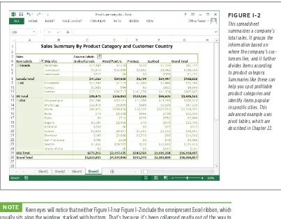
[image:17.504.60.463.128.443.2]The bottom line is that once you enter raw information, Excel’s built-in smarts can help compute all kinds of useful figures. Figure I-2 shows a sophisticated spreadsheet that’s designed to help identify hot-selling product categories.
FiGuRE i-2
This spreadsheet summarizes a company’s total sales. It groups the information based on where the company’s cus-tomers live, and it further divides items according to product category. Summaries like these can help you spot profitable product categories and identify items popular in specific cities. This advanced example uses pivot tables, which are described in Chapter 22.
NOTE Keen eyes will notice that neither Figure I-1 nor Figure I-2 include the omnipresent Excel ribbon, which usually sits atop the window, stacked with buttons. That’s because it’s been collapsed neatly out of the way to let you focus on the spreadsheet. You’ll learn how to use this trick yourself on page 15.
Excel is not just a math wizard. If you want to add a little life to your data, you can inject color, apply exotic fonts, and even create macros (automated sequences of steps) to help speed up repetitive formatting or editing chores. And if you’re bleary-eyed from staring at rows and rows of spreadsheet numbers, you can use Excel’s many chart-making tools to build everything from 3-D pie charts to more exotic scatter graphs. (See Chapter 17 to learn about all of Excel’s chart types.) Excel can be as simple or as sophisticated as you want it to be.
ThE nEW FEaTurEs in
ExCEl 2013 sources, from a data feed on a website to a database server in a big company. Once you bring that information into Excel, you can examine it with formulas and charts,
just as you would analyze the information in an ordinary workbook. You’ll see this side of Excel in Chapters 27 and 28.
The New Features in Excel 2013
For Excel 2007 and Excel 2010, Microsoft spent most of its time rebuilding the spreadsheet program’s user interface, replacing the clutter of old-fashioned toolbars with a unified ribbon, and creating a new backstage view where you can open, save, and print files. The visual changes in Excel 2013 are much less dramatic. Excel 2013 tweaks the program’s looks, but just a little, changing the capitalizing of toolbar tabs and toning down the color scheme. But the modern Excel window (which you’ll tour in Chapter 1) stays essentially the same.
That’s not to say that the creators of Excel haven’t been busy over the past few years. In fact, they’ve introduced a range of refinements and new features, most of which fall into two categories. First, Excel 2013 aims to be the easiest, most intuitive version of Excel yet, with several new features that offer help or make suggestions as you work with batches of data. Second, Excel 2013 has grown more powerful, so it can act as a data analysis tool for big businesses with boatloads of data.
You’ll learn about all of Excel’s changes in this book. Here’s a preview of the most significant new features:
• Flash Fill. Tired of making repetitive changes to a whole column of information? With Flash Fill, Excel watches you make minor changes, learns the pattern, and then offers to apply your edit to the rest of your data—automatically. You’ll put it to work on page 66.
• Quick Analysis. Excel always had plenty of great features, but you need to click your way through layers of buttons and menus to find them. But Excel’s new Quick Analysis feature gives you easy access to the most useful charting, summarizing, and data visualization options. Just select your data, click a simple smart tag, and pick one of the convenient choices Excel offers. Quick Analysis is particularly handy for basic charts (page 489), but you’ll see it crop up throughout this book.
ThE nEW FEaTurEs in
ExCEl 2013
• The new data model. Excel has always been a brilliant tool for pulling in data from a database and crunching the numbers. Now, Excel integrates the Power-Pivot add-in, giving it the ability to handle millions of rows of data. You’ll learn more in Chapter 27.
• Worksheet reporting. The Inquire add-in is a bonus that ships with the Office Professional Plus version of Excel. It lets you compare different versions of the same workbook, and discover how the formulas in sheets and workbook files link together, among other tricks. You’ll try it out on page 696.
Of course, this list is by no means complete. Excel 2013 is chock-full of refinements, tweaks, and tune-ups that make it easier to use than any previous version. You’ll learn all the best tricks throughout this book.
The Office 365 Subscription Service
Along with the changes covered above, Microsoft has been busy tweaking the way it sells Office. Excel 2013 is available in the usual array of desktop packages, as well as through a subscription service called Office 365, which is aimed at businesses, educational institutions, and government workers. When a company signs up, they give each of their employees a separate Office 365 account that they can use to run Office (either online or on the desktop, if the subscription plan includes desktop use). Depending on the plan, the Office 365 subscription may also include other online services, such as email, messaging, document sharing, project tracking, and more. The drawback to Office 365 is that each person who uses it needs a separate sub-scription plan, and each subsub-scription plan entails a monthly payment to Microsoft (ranging from $4 to over $20 per month). For big businesses, the cost of giving their employees Office 365 subscriptions is often less than buying multiple copies of the shrink-wrapped Office software, and it saves them many administrative tasks, be-cause Microsoft manages most of the administration, from spam filtering to setting up SharePoint. However, Office 365 probably won’t interest families, hobbyists, or self-employed people.
To learn more about Office 365 and compare the different subscription plans, visit
http://office.microsoft.com.
Office RT: Office for Tablets
Excel doesn’t just live on ordinary Windows PCs. Now, Microsoft gives Excel lovers a way to run their favorite program on a Windows 8 tablet (see below), or in a web browser (see the next section).
ThE nEW FEaTurEs in
ExCEl 2013 Office RT looks almost identical to the desktop version of Office, but it has a number of changes under the hood. For example, it’s optimized to conserve battery life and
save disk space. It also turns on touch mode, which makes it easier to scroll around and use the ribbon with your fingers instead of the traditional mouse pointer. Although this book is written with the full desktop version of Excel in mind, you can also use it to feel your way around the Office RT version of Excel. However, you’ll find that the instructions in this book are unashamedly mouse-centric (we talk about “right-clicking” but not “double-tapping,” for example). You should also know that there are a small set of significant Excel features that aren’t available in Office RT. These include macros, Visual Basic programming, plug-ins, and the new data model that lets you work with related tables and huge amounts of data.
NOTE Most Excel pros will continue to use desktop versions of Excel for hardcore spreadsheet work. They may switch to Office RT when they need to collect data on the go, or carry their latest analysis into a company meeting.
The Office Web Apps
The Office Web Apps are an interesting new direction in the Office world. They provide a way to run sophisticated Office applications, like Excel, in an ordinary browser and on virtually any computer. However, the Office Web Apps have only a sliver of the features of their desktop cousins, and you can’t use them at all unless you have a SharePoint server or you’re willing to upload your documents to SkyDrive (Microsoft’s free document-hosting service). The online version of Excel is called the Excel Web App.
NOTE Overall, the Excel Web App is designed for collecting data and viewing Excel spreadsheets, not creating them. For example, you can view workbooks that use common Excel ingredients like sparklines and pivot tables, but you can’t add them yourself.
Microsoft introduced the Excel Web App at the same time as Excel 2010. When the company released Excel 2013, they also updated the Excel Web App, giving it the new Excel 2013 color scheme and tweaking its chart drawing to be just a bit crisper. However, the only completely new feature you’ll find in the Excel 2013 Web App is the ability to create surveys (page 733).
abouT This book
About This Book
Despite the many improvements in software over the years, one feature hasn’t im-proved a bit: Microsoft’s documentation. In fact, with Office 2013, you get no printed user guide at all. To learn about the thousands of features included in this software collection, Microsoft expects you to read its online help.
Occasionally, the online help is actually helpful, like when you’re looking for a quick description explaining a mysterious new function. On the other hand, if you’re trying to learn how to, say, create an attractive chart, you’re stuck with terse and occasionally cryptic instructions.
The purpose of this book, then, is to serve as the manual that should have accom-panied Excel 2013. In these pages, you’ll find step-by-step instructions and tips for using almost every Excel feature, including those you may not even know exist.
About the Outline
This book is divided into eight parts, each containing several chapters.
• Part One: Worksheet Basics. In this part, you’ll get acquainted with Excel’s interface and learn the basic techniques for creating spreadsheets and entering and organizing data. You’ll also learn how to format your work to make it more presentable, and how to create sharp printouts.
• Part Two: Formulas and Functions. This part introduces you to Excel’s most important feature—formulas. You’ll learn how to perform calculations ranging from the simple to the complex, and you’ll tackle specialized functions for dealing with all kinds of information, including scientific, statistical, business, and financial data.
• Part Three: Organizing Your Information. The third part covers how to organize and find what’s in your spreadsheet. First, you’ll learn to search, sort, and filter large amounts of information by using tables. Next, you’ll see how to boil down complex tables using grouping and outlining. Finally, you’ll turn your perfected spreadsheets into reusable templates.
• Part Four: Charts and Graphics. The fourth part introduces you to charting and graphics, two of Excel’s most popular features. You’ll learn about the wide range of different chart types available and when it makes sense to use each one. You’ll also find out how you can use pictures to add a little pizazz to your spreadsheets.
abouT This
book • Part Six: Advanced Data Analysis.Excel’s most advanced features. You’ll see how to study different possibilities In this brief part, you’ll tackle some of
with scenarios, use goal-seeking and the Solver add-in to calculate “backward” and fill in missing numbers, and create multi-layered summary reports with pivot tables. You’ll also learn how to use Excel’s data connection features to pull information out of databases, websites, and XML files.
• Part Seven: Programming Excel. This part presents a gentle introduction to the world of Excel programming, first by recording macros and then by using the full-featured VBA (Visual Basic for Applications) language, which lets you automate complex tasks.
• Part Eight: Appendix. The end of this book wraps up with an appendix that shows you how to customize the ribbon to get easy access to your favorite commands.
About
>
These
>
Arrows
Throughout this book, you’ll find sentences like this one: “Choose Insert→Illustrations→
Picture.” This is a shorthand way of telling you how to find a feature in the Excel ribbon. It translates to the following instructions: “Click the Insert tab of the toolbar. On that tab, look for the Illustrations section. In the Illustrations box, click the Picture button.” Figure I-3 shows the button you want.
FiGuRE i-3
In this book, arrow notations help simplify ribbon commands. For example, “Choose Insert→ Illus-trations→Picture” leads to the highlighted button shown here.
abouT This book
CONTEXTUAL TABS
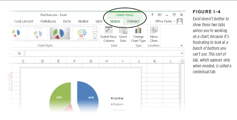
[image:23.504.61.462.113.317.2]There are some tabs that appear in the ribbon only when you work on specific tasks. For example, when you create a chart, a Chart Tools section appears with two new tabs (see Figure I-4).
FiGuRE i-4
Excel doesn’t bother to show these two tabs unless you’re working on a chart, because it’s frustrating to look at a bunch of buttons you can’t use. This sort of tab, which appears only when needed, is called a contextual tab.
When dealing with contextual tabs, the instructions in this book always include the title of the tab section (it’s Chart Tools in Figure I-4, for example). Here’s an exam-ple: “Choose Chart Tools | Design→Type→Change Chart Type.” Notice that the first
part of this instruction includes the tab section title (Chart Tools) and the tab name (Design), separated by the | character. That way, you can’t mistake the Chart Tools | Design tab for a Design tab in some other group of contextual tabs.
NOTE Excel adds contextual tabs after the standard tabs, so you’ll always see them on the right side of the Excel window.
BUTTONS WITH MENUS
abouT This book
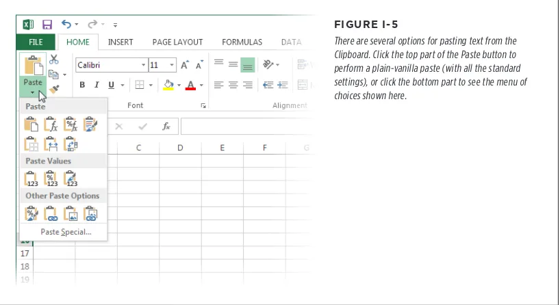
FiGuRE i-5
There are several options for pasting text from the Clipboard. Click the top part of the Paste button to perform a plain-vanilla paste (with all the standard settings), or click the bottom part to see the menu of choices shown here.
When dealing with this sort of button, the last step of the instructions in this book tells you what to choose from the drop-down menu. For example, say you’re direct-ed to “Home→Clipboard→Paste→Paste Special.” That tells you to select the Home
tab, look for the Clipboard section, click the drop-down part of the Paste button (to reveal the menu with extra options), and then choose Paste Special from the menu.
TIP Be on the lookout for drop-down arrows in the ribbon—they’re tricky at first. You need to click the arrow part of the button to see the full list of options. When you click any other part of the button, you don’t see the list. Instead, Excel fires off the standard command (the one Excel thinks is the most common choice) or the command you used most recently.
DIALOG BOX LAUNCHERS
abouT This book
The second way to get to a dialog box is through something called a dialog box launcher, which is just a nerdified name for the tiny square-with-arrow icon that sometimes appears in the bottom-right corner of a section of the ribbon. The easiest way to learn how to spot a dialog box launcher is to look at Figure I-6.
FiGuRE i-6
As you can see here, the Clipboard, Font, Alignment, and Number sections all have dialog box launchers. The Styles, Cells, and Editing sections don’t.
When you click a dialog box launcher, the related dialog box appears. For example, click the dialog box launcher for the Font section and you get a full Font dialog box that lets you scroll through all the typefaces on your computer, choose a size and color, and so on.
In this book, there’s no special code word that tells you to use a dialog box launch-er. Instead, you’ll see an instruction like this: “To see more font options, look at the Home→Font section and click the dialog box launcher (the small icon in the bottom-right corner).” Now that you know what a dialog box launcher is, that makes perfect sense.
BACKSTAGE VIEW
If you see an instruction that includes arrows but starts with the word File, it’s telling you to go to Excel’s backstage view. For example, the sentence “Choose File→New” means click the File button (which appears just to the left of ribbon’s Home tab) to switch to backstage view, then click the New command (which appears in the nar-row list on the left side of the window). You’ll take your first look around backstage view on page 23.
ORDINARY MENUS
onlinE
rEsourCEs
About Shortcut Keys
Every time you take your hand off the keyboard to move the mouse, you lose a few microseconds. That’s why many experienced computer fans use keystroke combi-nations instead of toolbars and menus wherever possible. Ctrl+S, for example, is a keyboard shortcut that saves your current work in Excel (and most other programs). When you see a shortcut like Ctrl+S in this book, it’s telling you to hold down the Ctrl key and, while it’s down, press the letter S, and then release both keys. Similarly, the finger-tangling shortcut Ctrl+Alt+S means hold down Ctrl, and then press and hold Alt, and then press S (so that all three keys are held down at once).
Online Resources
As the owner of a Missing Manual, you’ve got more than just a book to read. As you read this book, you’ll see a number of examples that demonstrate Excel features and techniques for building good spreadsheets. Most of these examples are available as downloadable Excel workbook files. Just surf to http://missingmanuals.com/cds/ excel2013mm/ to visit a page where you can download a ZIP file that includes the examples, organized by chapter.
Registration
If you register this book at www.oreilly.com, you’ll be eligible for special offers—like discounts on future editions of this book. If you buy the ebook from oreilly.com and register your purchase, you get free lifetime updates for this edition of the ebook; we’ll notify you by email when updates become available. Registering takes only a few clicks. Type www.oreilly.com/register into your browser to hop directly to the Registration page.
Feedback
Got questions? Need more information? Fancy yourself a book reviewer? On our Feed-back page, you can get expert answers to questions that come to you while reading, share your thoughts on this Missing Manual, and find groups for folks who share your interest in Dreamweaver. To have your say, go to www.missingmanuals.com/feedback.
Errata
onlinE rEsourCEs
Examples
As you read this book, you’ll see a number of examples that demonstrate Excel features and techniques for building good spreadsheets. Most of these examples are available as Excel workbook files in a separate download. Just surf to www.missingmanuals. com/cds and click the link for this book to visit a page where you can download a ZIP file that includes the examples, organized by chapter.
Safari
©Books Online
Safari© Books Online is an on-demand digital library that lets you easily search over 7,500 technology and creative reference books and videos to find the answers you need quickly.
With a subscription, you can read any page and watch any video from our library online. Read books on your cellphone and mobile devices. Access new titles before they’re available for print, and get exclusive access to manuscripts in development and post feedback for the authors. Copy and paste code samples, organize your favorites, download chapters, bookmark key sections, create notes, print out pages, and benefit from tons of other time-saving features.
Worksheet Basics
PART
1
CHAPTER 1
Creating Your First Spreadsheet
CHAPTER 2
Adding Information
CHAPTER 3
Moving Data Around
CHAPTER 4
Managing Worksheets
CHAPTER 5
Formatting Cells
CHAPTER 6
Smart Formatting Tricks
CHAPTER 7
ChAPTER
1
E
very Excel grandmaster needs to start somewhere. In this chapter, you’ll learn how to create a basic spreadsheet. First, you’ll find out how to move around Excel’s grid of cells, typing in numbers and text as you go. Next, you’ll take a quick tour of the Excel ribbon, the tabbed toolbar of commands that sits above your spreadsheet. You’ll learn how to trigger the ribbon with a keyboard shortcut, and collapse it out of the way when you don’t need it. Finally, you’ll go to Excel’s back-stage view, the file-management hub where you can save your work for posterity, open recent files, and tweak Excel options.Starting a Workbook
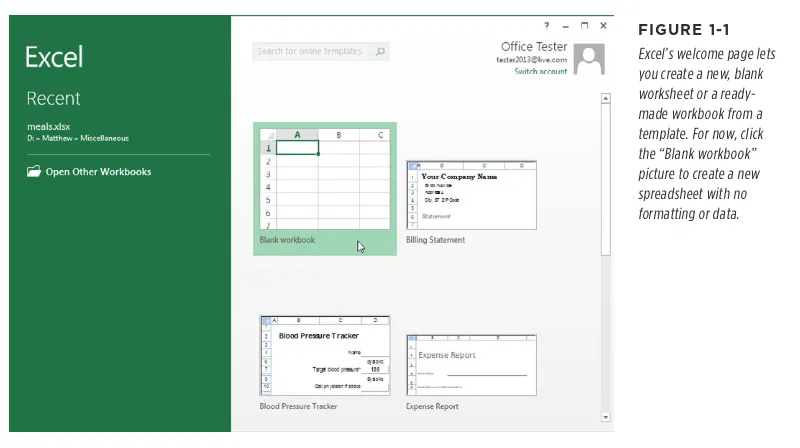
When you first fire up Excel, you’ll see a welcome page where you can choose to open an existing Excel spreadsheet or create a new one (Figure 1-1).
aDDing inForMaTion
[image:32.504.43.443.91.315.2]To a WorkshEET
FiGuRE 1-1
Excel’s welcome page lets you create a new, blank worksheet or a ready-made workbook from a template. For now, click the “Blank workbook” picture to create a new spreadsheet with no formatting or data.
Excel fills most of the welcome page with templates, spreadsheet files preconfigured for a specific type of data. For example, if you want to create an expense report, you might choose Excel’s “Travel expense report” template as a starting point. You’ll learn lots more about templates in Chapter 16, but for now, just click “Blank workbook” to start with a brand-spanking-new spreadsheet with no information in it.
NOTE Workbook is Excel lingo for “spreadsheet.” Excel uses this term to emphasize the fact that a single workbook can contain multiple worksheets, each with its own grid of data. You’ll learn about this feature in Chapter 4, but for now, each workbook you create will have just a single worksheet of information.
You don’t get to name your workbook when you first create it. That happens later, when you save your workbook (page 26). For now, you start with a blank canvas that’s ready to receive your numerical insights.
aDDing inForMaTion
[image:33.504.60.465.90.365.2]To a WorkshEET
FiGuRE 1-2
The largest part of the Excel window is the work-sheet grid, where you type in your information.
Here are a few basics about Excel’s grid:
• The grid divides your worksheet into rows and columns. Excel names columns using letters (A, B, C…), and labels rows using numbers (1, 2, 3…).
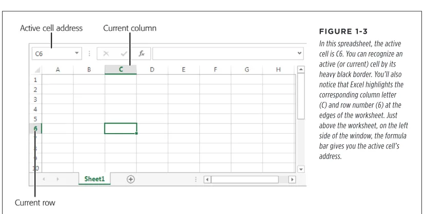
• The smallest unit in your worksheet is thecell. Excel uniquely identifies each cell by column letter and row number. For example, C6 is the address of a cell in column C (the third column) and row 6 (the sixth row). Figure 1-3 shows this cell, which looks like a rectangular box. Incidentally, an Excel cell can hold approximately 32,000 characters.
• A worksheet can span an eye-popping 16,000 columns and 1 million rows. In the unlikely case that you want to go beyond those limits—say, if you’re tracking blades of grass on the White House lawn—you’ll need to create a new worksheet. Every spreadsheet file can hold a virtually unlimited number of worksheets, as you’ll learn in Chapter 4.
aDDing inForMaTion
To a
[image:34.504.33.446.114.323.2]WorkshEET NOTE Obviously, once you go beyond 26 columns, you run out of letters. Excel handles this by doubling up (and then tripling up) letters. For example, after column Z is column AA, then AB, then AC, all the way to AZ and then BA, BB, BC—you get the picture. And if you create a ridiculously large worksheet, you’ll find that column ZZ is followed by AAA, AAB, AAC, and so on.
FiGuRE 1-3
In this spreadsheet, the active cell is C6. You can recognize an active (or current) cell by its heavy black border. You’ll also notice that Excel highlights the corresponding column letter (C) and row number (6) at the edges of the worksheet. Just above the worksheet, on the left side of the window, the formula bar gives you the active cell’s address.
The best way to get a feel for Excel is to dive right in and start putting together a worksheet. The following sections cover each step that goes into assembling a simple worksheet. This one tracks household expenses, but you can use the same approach with any basic worksheet.
Adding Column Titles
Excel lets you arrange information in whatever way you like. There’s nothing to stop you from scattering numbers left and right, across as many cells as you want. However, one of the most common (and most useful) ways to arrange information is in a table, with headings for each column.
aDDing inForMaTion
[image:35.504.59.458.89.370.2]To a WorkshEET
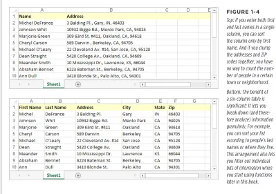
FiGuRE 1-4
Top: If you enter both first and last names in a single column, you can sort the column only by first name. And if you clump the addresses and ZIP codes together, you have no way to count the num-ber of people in a certain town or neighborhood. Bottom: The benefit of a six-column table is significant: It lets you break down (and there-fore analyze) information granularly, For example, you can sort your list according to people’s last names or where they live. This arrangement also lets you filter out individual bits of information when you start using functions later in this book.
You can, of course, always add or remove columns. But you can avoid getting gray hairs by starting a worksheet with all the columns you think you’ll need.
The first step in creating a worksheet is to add your headings in the row of cells at the top of the sheet (row 1). Technically, you don’t need to start right in the first row, but unless you want to add more information before your table—like a title for the chart or today’s date—there’s no point in wasting space. Adding information is easy—just click the cell you want and start typing. When you finish, hit Tab to complete your entry and move to the cell to the right, or click Enter to head to the cell just underneath.
aDDing inForMaTion
To a
WorkshEET For a simple expense worksheet designed to keep a record of your most prudent and extravagant purchases, try the following three headings:
• Date Purchased. Stores the date when you spent the money. • Item. Stores the name of the product that you bought. • Price. Records how much it cost.
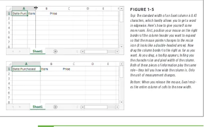
[image:36.504.36.445.173.429.2]Right away, you face your first glitch: awkwardly crowded text. Figure 1-5 shows how to adjust the column width for proper breathing room.
FiGuRE 1-5
Top: The standard width of an Excel column is 8.43 characters, which hardly allows you to get a word in edgewise. Here’s how to give yourself some more room. First, position your mouse on the right border of the column header you want to expand so that the mouse pointer changes to the resize icon (it looks like a double-headed arrow). Now drag the column border to the right as far as you want. As you drag, a tooltip appears, telling you the character size and pixel width of the column. Both of these pieces of information play the same role—they tell you how wide the column is. Only the unit of measurement changes.
Bottom: When you release the mouse, Excel resiz-es the entire column of cells to the new width.
NOTE A column’s character width doesn’t really reflect how many characters (or letters) fit in a cell. Excel uses proportional fonts, in which different letters take up different amounts of room. For example, the letter W is typically much wider than the letter I. All this means is that the character width Excel shows you isn’t a real indication of how many letters can fit in the column, but it’s a useful way to compare column widths.
Adding Data
aDDing inForMaTion
To a WorkshEET
FiGuRE 1-6
This rudimentary expense list has three items in it (in rows 2, 3, and 4). By default, Excel aligns the items in a column according to their data type. It aligns numbers and dates on the right, and text on the left.
That’s it. You’ve now created a living, breathing worksheet. The next section explains how you can edit the data you just entered.
Editing Data
Every time you start typing in a cell, Excel erases any existing content in that cell. (You can also quickly remove the contents of a cell by moving to the cell and pressing Delete, which clears its contents.)
If you want to edit cell data instead of replacing it, you need to put the cell in edit mode, like this:
1. Move to the cell you want to edit.
Use the mouse or the arrow keys to get to the correct cell.
2. Put the cell in edit mode by pressing F2 or by double-clicking inside it. Edit mode looks like ordinary text-entry mode, but you can use the arrow keys to position your cursor in the text you’re editing. (When you aren’t in edit mode, pressing these keys just moves you to another cell.)
3. Complete your edit.
Once you modify the cell content, press Enter to confirm your changes or Esc to cancel your edit and leave the old value in the cell. Alternatively, you can click on another cell to accept the current value and go somewhere else. But while you’re in edit mode, you can’t use the arrow keys to move out of the cell.
aDDing inForMaTion
To a
WorkshEET As you enter data, you may discover the Bigtime Excel Display Problem (known to aficionados as BEDP): Cells in adjacent columns can overlap one another. Figure
[image:38.504.34.444.350.568.2]1-7 illustrates the problem. One way to fix BEDP is to manually resize the column, as shown in Figure 1-5. Another option is to turn on text wrapping so you can fit multiple lines of text in a single cell, as described on page 151.
FiGuRE 1-7
Overlapping cells can create big head-aches. For example, if you type a large amount of text into A1 and then you type some text into B1, you see only part of A1’s data in your worksheet (as shown here). The rest is hidden from view. But if, say, A3 contains a large amount of text and B3 is empty, Excel displays the content in A3 over both columns, and you don’t have a problem.
Editing Cells with the Formula Bar
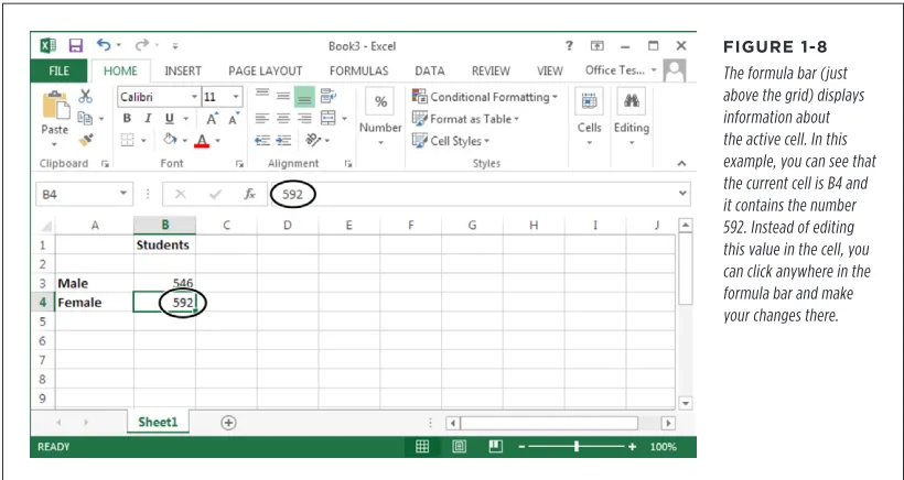
Just above the worksheet grid but under the ribbon is an indispensable editing tool called the formula bar (Figure 1-8). It displays the address of the active cell (like A1) on the left edge, and it shows you the current cell’s contents.
FiGuRE 1-8
aDDing inForMaTion
To a WorkshEET
[image:39.504.59.460.205.462.2]You can use the formula bar to enter and edit data instead of editing directly in your worksheet. This is particularly useful when a cell contains a formula or a large amount of information. That’s because the formula bar gives you more work room than a typical cell. Just as with in-cell edits, you press Enter to confirm formula bar edits or Esc to cancel them. Or you can use the mouse: When you start typing in the formula bar, a checkmark and an “X” icon appear just to the left of the box where you’re typing. Click the checkmark to confirm your entry or “X” to roll it back. Ordinarily, the formula bar is a single line. If you have a really long entry in a cell (like a paragraph’s worth of text), you need to scroll from one side to the other. However, there’s another option—you can resize the formula bar so that it fits more information, as shown in Figure 1-9.
FiGuRE 1-9
using ThE ribbon
POWER USERS’ CLINIC
Using R1C1 Reference Style
Most people like to identify columns with letters and rows with numbers. This system makes it easy to tell the difference between the two, and it lets you use short cell addresses like A10, B4, and H99. When you first install Excel, it uses this style of cell addressing.
However, Excel lets you use another cell addressing system called R1C1. In R1C1 style, Excel identifies both rows and columns with numbers. That means the cell address A10 becomes R10C1 (read this as Row 10, Column 1). The letters R and C tell you which part of the address represents the row number and which part is the column number. The R1C1 format reverses the order of conventional cell addressing.
R1C1 addressing isn’t all that common, but it can be useful if you need to deal with worksheets that have more than 26 columns. With normal cell addressing, Excel runs out of letters after column 26, and it starts using two-letter column names (as in AA, AB, and so on). But this approach can get awkward.
For example, if you want to find cell AX1, it isn’t immediately obvious that cell AX1 is in column 50. On the other hand, the R1C1 address for the same cell—R1C50—gives you a clearer idea of where to find the cell.
To use R1C1 for a spreadsheet, select File→Options. This shows the Excel Options window, where you can change a wide array of settings. In the list on the left, choose Formulas to hone in on the section you need. Then, look under the “Working with formulas” heading, and turn on the “R1C1 reference style” checkbox.
R1C1 is a file-specific setting, which means that if someone sends you a spreadsheet saved using R1C1, you’ll see the R1C1 cell addresses when you open the file, regardless of what type of cell addressing you use in your own spreadsheets. Fortunately, you can change cell addressing at any time using the Excel Options window.
Using the Ribbon
The focal point of the Excel window is the worksheet grid. It’s where you enter and edit information, whether that’s an amortization table for a business loan or a cat-alog of your rare Spider-Man comics. However, it won’t be long before you need to direct your attention upwards, to the super-toolbar that sits at the top of the Excel window. This is the ribbon, and it ensures that even the geekiest Excel features are only a click or two away.
The Tabs of the Ribbon
using ThE ribbon
FiGuRE 1-10
When you launch Excel, you start at the Home tab. But here’s what happens when you click the Page Layout tab. Now, you have a slew of options for tasks like adjusting paper size and making a decent printout. Excel groups the buttons within a tab into smaller sections for clearer organization.
using ThE ribbon
FiGuRE 1-11
Top: A large Excel window gives you plenty of room to play. The ribbon uses the space effectively, making the most import-ant buttons bigger. Bottom: When you shrink the Excel window, the ribbon shrinks some buttons or hides their text to make room. Shrink small enough, and Excel starts to replace cramped sections with a single button, like the Alignment, Cells, and Editing sections shown here. Click the button and the missing commands appear in a drop-down panel.
Throughout this book, you’ll dig through the ribbon’s tabs to find important features. But before you start your journey, here’s a quick overview of what each tab provides.
• File isn’t really a toolbar tab, even though it appears first in the list. Instead, it’s your gateway to Excel’s backstage view, as described on page 23.
• Home includes some of the most commonly used buttons, like those for cutting and pasting text, formatting data, and hunting down important information with search tools.
• Insert lets you add special ingredients to your spreadsheets, like tables, graphics, charts, and hyperlinks.
• Page Layout is all about getting your worksheet ready for printing. You can tweak margins, paper orientation, and other page settings.
using ThE ribbon
• Review includes the familiar Office proofing tools (like the spell-checker). It also has buttons that let you add comments to a worksheet and manage revisions. • View lets you switch on and off a variety of viewing options. It also lets you pull
off a few fancy tricks if you want to view several separate Excel spreadsheet files at the same time; see page 200.
NOTE In some circumstances, you may see tabs that aren’t in this list. Macro programmers and other highly technical types use the Developer tab. (You’ll learn how to reveal this tab on page 916.) The Add-Ins tab appears when you open workbooks created in previous versions of Excel that use custom toolbars. And finally, you can create a tab of your own if you’re ambitious enough to customize the ribbon, as explained in the Appendix.
Collapsing the Ribbon
Most people are happy to have the ribbon sit at the top of the Excel window, with all its buttons on hand. But serious number-crunchers demand maximum space for their data—they’d rather look at another row of numbers than a pumped-up tool-bar. If this describes you, then you’ll be happy to find out that you can collapse the ribbon, which shrinks it down to a single row of tab titles, as shown in Figure 1-12. To collapse it, just double-click the current tab title. (Or click the tiny up-pointing icon in the top-right corner of the ribbon, right next to the help icon.)
FiGuRE 1-12
Do you want to use every square inch of screen space for your cells? You can collapse the ribbon (as shown here) by double-clicking any tab. Click a tab to pop it open temporarily, or double-click a tab to bring the ribbon back for good. And if you want to perform the same trick without lifting your fin-gers from the keyboard, use the shortcut Ctrl+F1.
using ThE
ribbon If you use the ribbon only occasionally, or if you prefer to use keyboard shortcuts, it makes sense to collapse the ribbon. Even then, you can still use the ribbon
com-mands—it just takes an extra click to open the tab. On the other hand, if you make frequent trips to the ribbon or you’re learning about Excel and like to browse the ribbon to see what features are available, don’t bother collapsing it. The two or three spreadsheet rows you’ll lose are well worth it.
Using the Ribbon with the Keyboard
If you’re an unredeemed keyboard lover, you’ll be happy to hear that you can trig-ger ribbon commands with the keyboard. The trick is using keyboard accelerators, a series of keystrokes that starts with the Alt key (the same key you used to use to get to a menu). When you use a keyboard accelerator, you don’t hold down all the keys at the same time. (As you’ll soon see, some of these keystrokes contain so many letters that you’d be playing Finger Twister if you tried.) Instead, you hit the keys one after the other.
The trick to keyboard accelerators is understanding that once you hit the Alt key, there are two things you do, in this order:
1. Pick the ribbon tab you want. 2. Choose a command in that tab.
Before you can trigger a specific command, you must select the correct tab (even if it’s already selected). Every accelerator requires at least two key presses after you hit the Alt key. You need to press even more keys to dig through submenus. By now, this whole process probably seems hopelessly impractical. Are you really expected to memorize dozens of accelerator key combinations?
using ThE ribbon
FiGuRE 1-13
When you press Alt, Excel displays KeyTips next to every tab, over the File menu, and over the but-tons in the Quick Access toolbar. If you follow up with M (for the Formulas tab), you’ll see letters next to every command in that tab, as shown in Figure 1-11.
FiGuRE 1-14
You can now follow up with F to trigger the Insert Function button, U to get to the AutoSum feature, and so on. Don’t bother trying to match letters with tab or button names—there are so many features packed into the ribbon that in many cases the letters don’t mean anything at all.
Sometimes, a command might have two letters, in which case you need to press both keys, one after the other. (For example, the Find & Select button on the Home tab has the letters FD. To trigger it, press Alt, then H, then F, and then D.)
using ThE
ribbon Excel gives you other shortcut keys that don’t use the ribbon. These are key com-binations that start with the Ctrl key. For example, Ctrl+C copies highlighted text,
and Ctrl+S saves your work. Usually, you find out about a shortcut key by hovering over a command with your mouse. For example, hover over the Paste button in the ribbon’s Home tab, and you see a tooltip that tells you its timesaving shortcut key, Ctrl+V. And if you worked with a previous version of Excel, you’ll find that Excel 2013 uses almost all the same shortcut keys.
NOSTALGIA CORNER
Excel 2003 Menu Shortcuts
If you’ve worked with an old version of Excel, you might have trained yourself to use menu shortcuts—key combinations that open a menu and pick out the command you want. For example, if you press Alt+E in Excel 2003, the Edit menu pops open. You can then press the S key to choose the Paste Special command. At first glance, it doesn’t look like these keyboard shortcuts will amount to much in Excel 2013. After all, Excel 2013 doesn’t even have a corresponding series of menus! Fortunately, Microsoft went to a little extra trouble to make life easier for longtime Excel aficionados. The result is that you can still use your menu shortcuts, but they work in a slightly different way.
When you hit Alt+E in Excel 2013, you see a tooltip appear over the top of the ribbon (Figure 1-15) that lets you know you’ve started to enter an Excel 2003 menu shortcut. If you go on to press S, you wind up at the familiar Paste Special window, because Excel knows what you’re trying to do. It’s almost as though Excel has an invisible menu at work behind the scenes. Of course, this feature can’t help you out all the time. It doesn’t work if you try to use one of the few commands that don’t exist any longer. And if you need to see the menu to remember what key to press next, you’re out of luck. All Excel gives you is the tooltip.
FiGuRE 1-15
using ThE sTaTus bar
The Quick Access Toolbar
Keen eyes will have noticed the tiny bit of screen real estate just above the ribbon. It holds a series of tiny icons, like the toolbars in older versions of Excel (Figure 1-16). This is the Quick Access toolbar (or QAT, to Excel nerds).
FiGuRE 1-16
The Quick Access toolbar puts the Save, Undo, and Redo commands right at your fingertips. Excel provides easy access to these commands because most people use them more frequently than any others. But as you’ll learn in the Appendix, you can add any commands you want here.
If the Quick Access toolbar were nothing but a specialized shortcut for three com-mands, it wouldn’t be worth the bother. But it has one other notable attribute: You can customize it. In other words, you can remove commands you don’t use and add your own favorites. The Appendix of this book (page 945) shows you how. Microsoft has deliberately kept the Quick Access toolbar very small. It’s designed to provide a carefully controlled outlet for those customization urges. Even if you go wild stocking the Quick Access toolbar with your own commands, the rest of the ribbon remains unchanged. (And that means a co-worker or spouse can still use Excel, no matter how dramatically you change the QAT.)
Using the Status Bar
using ThE sTaTus bar
FiGuRE 1-17
In the status bar, you can see the basic status text (which just says “Ready” in this example), the view buttons (useful as you prepare a spreadsheet for printing), and the zoom slider (which lets you enlarge or shrink the current worksheet).
The status bar combines several types of information. The leftmost area shows Cell Mode, which displays one of three indicators:
• Ready means that Excel isn’t doing anything much at the moment, other than waiting to execute a command.
• Enter appears when you start typing a new value into a cell.
• Edit means you currently have the cell in edit mode, and pressing the left and right arrow keys moves through the data within a cell, instead of moving from cell to cell. You can place a cell in edit mode or take it out of edit mode by pressing F2.
Farther to the right of the status bar are the view buttons, which let you switch to Page Layout view or Page Break Preview. These help you see what your worksheet will look like when you print it. They’re covered in Chapter 7.
The zoom slider is next to the view buttons, at the far right edge of the status bar. You can slide it to the left to zoom out (which fits more information into your Excel window) or slide it to the right to zoom in (and take a closer look at fewer cells). You can learn more about zooming on page 190.
using ThE sTaTus bar
TABlE 1-1 Status bar indicators
INDICATOR MEANING
Cell Mode Shows Ready, Edit, or Enter depending on the state of the current cell.
Flash Fill Blank Cells and Flash Fill Changed Cells
Shows the number of cells that were skipped (left blank) and the number of cells that were filled after a Flash Fill operation (page 65).
Signatures, Information Management Policy, and Permissions
Displays information about the rights and restrictions of the current spreadsheet. These features come into play only if you use a SharePoint server to share spreadsheets among groups of people (usually in a corporate environment).
Caps Lock Indicates whether you have Caps Lock mode on. When it is, Excel automatically capitalizes every letter you type. To turn Caps Lock on or off, hit the Caps Lock key.
Num Lock Indicates whether Num Lock mode is on. When it is, you can use the numeric keypad (typically on the right side of your keyboard) to type in numbers more quickly. When this sign’s off, the numeric keypad controls cell navigation instead. To turn Num Lock on or off, press Num Lock.
Scroll Lock Indicates whether Scroll Lock mode is on. When it’s on, you can use the arrow keys to scroll through a worksheet without changing the active cell. (In other words, you can control your scrollbars by just using your keyboard.) This feature lets you look at all the information in your worksheet without losing track of the cell you’re currently in. You can turn Scroll Lock mode on or off by pressing Scroll Lock.
Fixed Decimal Indicates when Fixed Decimal mode is on. When it is, Excel automatically adds a set number of decimal places to the values you enter in any cell. For example, if you tell Excel to use two fixed decimal places and you type the number 5 into a cell, Excel actually enters 0.05. This seldom-used featured is handy for speed typists who need to enter reams of data in a fixed format. You can turn this feature on or off by selecting File→Options, choosing the Advanced section, and then looking
under “Editing options” to find the “Automatically insert a decimal point” setting. Once you turn this checkbox on, you can choose the number of decimal places displayed (the standard option is 2).
using ThE
sTaTus bar INDICATOR MEANING
End Mode Indicates that you’ve pressed End, which is the first key in many two-key combinations; the next key determines what happens. For example, hit End and then Home to move to the bottom-right cell in your worksheet.
Macro Recording Macros are automated routines that perform some task in an Excel spreadsheet. The Macro Recording indicator shows a record button (which looks like a red circle superimposed on a worksheet) that lets you start recording a new macro. You’ll learn more about macros in Chapter 29.
Selection Mode Indicates the current Selection mode. You have two options: normal mode and extended selection. When you press the arrows keys with Extended selection on, Excel automatically selects all the rows and columns you cross as you move around the spreadsheet. Extended selection is a useful keyboard alternative to dragging your mouse to select swaths of the grid. To turn Extended selection on or off, press F8. You’ll learn more about selecting cells and moving them around in Chapter 3. Page Number Shows the current page and the total number of pages (as in
“page 2 of 4”). This indicator appears only in Page Layout view (as described on page 209).
Average, Count, Numerical Count, Minimum, Maximum, Sum
Show the result of a calculation on selected cells. For exam-ple, the Sum indicator totals the value of all the numeric cells selected. You’ll take a closer look at this handy trick on page 88. Upload Status Does nothing (that we know of). Excel does show a handy
indi-cator in the status bar when you’re uploading files to the Web, as you’ll learn in Chapter 26. However, Excel always displays the upload status when needed, and this setting doesn’t seem to have any effect.
View Shortcuts Shows the three view buttons that let you switch between Normal view, Page Layout view, and Page Break Preview. Zoom Shows the current zoom percentage (like 100 percent for a
normal-sized spreadsheet, and 200 percent for a spreadsheet that’s blown up to twice the magnification).
going baCksTagE
FiGuRE 1-18
Every item that has a checkmark appears in the status bar when you need it. For example, if you choose Caps Lock, the text “Caps Lock” appears in the status bar whenever you hit the Caps Lock key. The text that appears on the right side of the list tells you the current value of the indicator. In this example, Caps Lock mode is currently off and the Cell Mode text says “Ready.”
Going Backstage
Your data is the star of the show. That’s why the creators of Excel refer to your worksheet as being “on stage.” The auditorium is the Excel main window, which—as you’ve just seen—includes the handy ribbon, formula bar, and status bar. Sure, it’s a strange metaphor. But once you understand it, you’ll realize the rationale for Excel’s
going
baCksTagE To switch to backstage view, click the File button to the left of the Home ribbon tab. Excel temporarily tucks your worksheet out of sight (although it’s still open and
[image:52.504.38.443.137.369.2]waiting for you). This gives Excel the space it needs to display information related to the task at hand, as shown in Figure 1-19. For example, if you plan to print your spreadsheet, Excel’s backstage view previews the printout. Or if you want to open an existing spreadsheet, Excel can display a detailed list of files you recently worked on.
FiGuRE 1-19
When you first switch to backstage view, Excel shows the Info page, which provides basic information about your workbook file, its size, when it was last edited, who edited it, and so on (see the column on the far right). The Info page also provides the gateway to three important features: document pro-tection (Chapter 21), com-patibility checking (page 31), and AutoRecover backups (page 38). To go to another section, click a different command in the column on the far left.
To get out of backstage view and return to your worksheet, press Esc or click the arrow-in-a-circle icon in the top-right corner of backstage view.
The key to using backstage view is the menu of commands that runs in a strip along the left side of the window. You click a command to get to the page for the task you want to perform. For example, to create a new spreadsheet (in addition to the one you’re currently working on), you begin by clicking the New command, as shown in Figure 1-20.
going baCksTagE
FiGuRE 1-20
When you click New, you see a page resembling the welcome page that greets you when you start Excel. To create a new, empty workbook, click “Blank workbook.” Excel opens the workbook in a new window, so that it’s separate from your current workbook, which Excel leaves untouched.
Here are some of the things you’ll do in Excel’s backstage view:
• Workwith files (create, open, close, and save them) with the help of the New, Open, Save, and Save As commands. You’ll spend the rest of this chapter learning the fastest and most effective ways to save and open Excel files.
• Print your work (Chapter 7) and email it to other people (Chapter 25) using the Print and Share commands.
• Prepare a workbook you want to share with others. For example, you can check its compatibility with older versions of Excel (Chapter 1) and lock your document to prevent other people from changing numbers (Chapter 24). You find these options under the Info command.
• Configureyour Office account—that’s the email address and password you use to access Microsoft’s SkyDrive service for storing spreadsheets online (page 706) or for your Office 365 account (if you’re a subscriber; see page xvii). To do this, click the Account command.
saving FilEs
Saving Files
As everyone who’s been alive for at least three days knows, you should save your work early and often. Excel is no exception. To save a file for the first time, choose File→Save or File→Save As. Either way, you end up at the Save As page in backstage
[image:54.504.40.444.136.372.2]view (Figure 1-21).
FiGuRE 1-21
The first time you save your spreadsheet, you need to choose where to put it. Usually, you’ll pick a location on your hard drive (click Computer in the Places list), but you can upload it to a corpo-rate SharePoint service or to Microsoft’s SkyDrive for online sharing almost as easily.
The Save As window includes a list of places—locations where you can store your work. The exact list depends on how you configured Excel, but here are some of the options you’re likely to see:
saving FilEs
FiGuRE 1-22
Once you pick a location for your file, you need to give it a name. This window won’t surprise you, because it’s the same Save As window that puts in an appearance in almost every document-based Windows application.
• SkyDrive. When you set up Excel, you can supply the email address and pass-word you use for Microsoft services like Hotma