Essentials of Theoretical Computer Science F D Lewis pdf

s

Essentials

of

heoretic

Theoretical

ter

Computer

nc

Science

F. D. Lewis

University of Kentucky

How to Navigate

O

CONTENTS

Copyright Notice Preface

COMPUTABILITY

The NICE Programming Language Turing Machines

A Smaller Programming Language Equivalence of the Models

Machine Enhancement

The Theses of Church and Turing

Historical Notes and References Problems

UNSOLVABILITY

Properties of the Enumeration Universal Machines and Simulation Solvability and the Halting Problem Reducibility and Unsolvability Enumerable and Recursive Sets

Historical Notes and References Problems

COMPLEXITY

Measures and Resource Bounds Complexity Classes

Reducibilities and Completeness The Classes P and NP

Intractable Problems

Finite Automata Closure Properties

Nondeterministic Operation Regular Sets and Expressions

Decision Problems for Finite Automata Pushdown Automata

Unsolvable Problems for Pushdown Automata Linear Bounded Automata

Historical Notes and References Problems

LANGUAGES

Language Properties Regular Languages Context Free Languages

Context Free Language Properties Parsing and Deterministic Languages Summary

C

P

B

Y

COMPUTABILITY

Before examining the intrinsic nature of computation we must have a precise idea of what computation means. In other words, we need to know what we’re talking about! To do this, we shall begin with intuitive notions of terms such as calculation, computing procedure, and algorithm. Then we shall be able to develop a precise, formal characterization of computation which captures all of the modern aspects and concepts of this important activity.

Part of this definitional process shall involve developing models of computation. They will be presented with emphasis upon their finite nature and their computational techiques, that is, their methods of transforming inputs into outputs. In closing, we shall compare our various models and discuss their relative power.

The sections are entitled:

The NICE Programming Language Turing Machines

A Smaller Programming Language Equivalence of the Models

Machine Enhancement

As computer scientists, we tend to believe that computation takes place inside computers. Or maybe computations are the results from operating computing machinery. So, when pressed to describe the limits of computation we might, in the spirit of Archimedes and his lever, reply that anything can be computed given a large enough computer! When pressed further as to how this is done we probably would end up by saying that all we need in order to perform all possible computations is the ability to execute programs which are written in some marvelous, nonrestrictive programming language. A nice one!

Since we are going to study computation rather than engage in it, an actual computer is not required, just the programs. These shall form our model of computation. Thus an ideal programming language for computation seems necessary. Let us call this the NICE language and define it without further delay. Then we can go on to describing what is meant by computation.

We first need the raw materials of computation. Several familiar items come immediately to mind. Numbers (integers as well as real or floating point) and Boolean constants (true and false) will obviously be needed. Our programs shall then employ variables that take these constants as values. And since it is a good idea to tell folks exactly what we're up to at all times, we shall declare these variables before we use them. For example:

var x, y, z: integer; p, q: Boolean; a, b, c: real;

Here several variables have been introduced and defined as to type. Since the world is often nonscalar we always seem to want some data structures. Arrays fill that need. They may be multidimensional and are declared as to type and dimension. Here is an array declaration.

var d, e: array[ , ] of integer; s: array[ ] of real;

We note that s is a one-dimensional array while h has four dimensions. As is usual in computer science, elements in arrays are referred to by their position. Thus s[3] is the third element of the array named s.

So far, so good. We have placed syntactic restrictions upon variables and specified our constants in a rather rigid (precise?) manner. But we have not placed any bounds on the magnitude of numbers or array dimensions. This is fine since we did not specify a particular computer for running the programs. In fact, we are dealing with ideal, gigantic computers that can handle very large values. So why limit ourselves? To enumerate:

a) Numbers can be of any magnitude.

b) Arrays may be declared to have as many dimensions as we wish.

c) Arrays have no limit on the number of elements they contain.

Our only restriction will be that at any instant during a computation everything must be finite. That means no numbers or arrays of infinite length. Huge - yes, but not infinite! In particular, this means that the infinite decimal expansion 0.333... for one third is not allowed yet several trillion 3's following a decimal point is quite acceptable. We should also note that even though we have a number type named real, these are not real numbers in the mathematical sense, but floating point numbers.

On to the next step - expressions. They are built from variables, constants, operators, and parentheses. Arithmetic expressions such as these:

x + y∗(z + 17) a[6] - (z∗b[k, m+2])/3

may contain the operators for addition, subtraction, multiplication, and division. Boolean expressions are formed from arithmetic expressions and relational operators. For example:

x + 3 = z/y -17 a[n] > 23

Compound Boolean expressions also contain the logical connectives and, or, and not. They look like this:

x - y > 3 and b[7] = z and v (x = 3 or x = 5) and not z = 6

In every programming language computational directives appear as statements. Our NICE language contains these also. To make things a little less wordy we shall introduce some notation. Here is the master list:

E arbitrary expressions AE arithmetic expressions BE Boolean expressions V variables

S arbitrary statements N numbers

Variables, statements, and numbers may be numbered (V6, S1, N9) in the descriptions of some of the statements used in NICE programs that follow.

a) Assignment. Values of expressions are assigned to variables in statements of the form: V = E.

b) Transfer. This statement takes the form goto N where N is an integer which is used as a label. Labels precede statements. For example: 10: S.

c) Conditional. The syntax is: if BE then S1 else S2 where the else clause is optional.

d) Blocks. These are groups of statements, separated by semicolons and bracketed by begin and end. For example: begin S1; S2; … ; Sn end

Figure 1 contains a fragment of code that utilizes every statement defined so far. After executing the block, z has taken on the value of x factorial.

begin

z = 1; 10: z = z*x; x = x - 1;

if not x = 0 then goto 10 end

Figure 1- Factorial Computation

e) Repetition. The while and for statements cause repetition of other statements and have the form:

Steps in a for statement are assumed to be one unless downto (instead of to) is employed. Then the steps are minus one as then we decrement rather than increment. It is no surprise that repetition provides us with structured ways to compute factorials. Two additional methods appear in figure 2.

begin z = 1;

for n = 2 to x do z = z*n end

begin z = 1; n = 1;

while n < x do begin

n = n + 1; z = z*n end

end

Figure 2 - Structured Programming Factorial Computation

f) Computation by cases. The case statement is a multiway, generalized if statement and is written:

case AE of N1: S1; N2: S2; ... ; Nk: Sk endcase

where the Nk are numerical constants. It works in a rather straightforward manner. The expression is evaluated and if its value is one of the Nk, then the corresponding statement Sk is executed. A simple table lookup is provided in figure 3. (Note that the cases need not be in order nor must they include all possible cases.)

case x - y/4 of: 15: z = y + 3; 0: z = w*6; 72: begin

x = 7; z = -2*z end;

6: w = 4 endcase

Figure 3 - Table Lookup

Now that we know all about statements and their components it is time to define programs. We shall say that a program consists of a heading, a declaration section and a statement (which is usually a block). The heading looks like:

program name(V1, V2, ... , Vn)

and contains the name of the program as well as its input parameters. These parameters may be variables or arrays. Then come all of the declarations followed by a statement. Figure 4 contains a complete program.

program expo(x, y)

var n, x, y, z: integer; begin

z = 1;

for n = 1 to y do z = z*x; halt(z)

end

Figure 4 - Exponentiation Program

The only thing remaining is to come to an agreement about exactly what programs do. Let's accomplish this by examining several. It should be rather obvious that the program of figure 4 raises x to the y-th power and outputs this value. So we shall say that programs compute functions.

Our next program, in figure 5, is slightly different in that it does not return a numerical value. Examine it.

program square(x) var x, y: integer; begin

y = 0;

while y*y < x do y = y + 1;

if y*y = x then halt(true) else halt(false) end

Figure 5 - Boolean Function

This program does return an answer, so it does compute a function. But it is a Boolean function since it returns either true or false. We depict this one as:

Or, we could say that the program named ‘square’ decides whether or not an integer is a perfect square. In fact, we state that this program decides membership for the set of squares.

Let us sum up all of the tasks we have determined that programs accomplish when we execute them. We have found that they do the following two things.

a) compute functions

b) decide membership in sets

And, we noted that (b) is merely a special form of (a). That is all we know so far.

So far, so good. But, shouldn’t there be more? That was rather simple. And, also, if we look closely at our definition of what a program is, we find that we can write some strange stuff. Consider the following rather silly program.

program nada(x) var x, y: integer; x = 6

Is it a program? Well, it has a heading, all of the variables are declared, and it ends with a statement. So, it must be a program since it looks exactly like one. But, it has no halt statement and thus can have no output. So, what does it do? Well, not much that we can detect when we run it!

Let's try another in the same vein. Consider the well-known and elegant:

program loop(x) var x: integer;

while x = x do x = 17

which does something, but alas, nothing too useful. In fact, programs which either do not execute a halt or even contain a halt statement are programs, but accomplish very little that is evident to an observer. We shall say that these compute functions which are undefined (one might say that f(x) = ?) since we do not know how else to precisely describe the results attained by running them.

program fu(x)

var n, x: integer; begin

n = 0;

while not x = n do n = n - 2; halt(x)

end

Figure 6 - A Partially Defined Function

This halts only for even, positive integers and computes the function described as:

fu(x) = x if x is even and positive, otherwise undefined

When a program does not halt, we shall say it diverges. The function fu could also be defined using mathematical notation as follows.

   =

otherwise diverge

positive and

even is x if x fu(x)

Since it halts at times (and thus is defined on the even, positive integers) we will compromise and maintain that it is partially defined.

To recap, we have agreed that computation takes place whenever programs are run on some ideal machine and that programs are written according to the rules of our NICE language.

An important note is needed here. We have depended heavily upon our computing background for the definition of exactly what occurs when computation takes place rather than dwell upon the semantics of the NICE language. We could go into some detail of how statements in our language modify the values of variables and so forth, but have agreed not to at this time.

So, given that we all understand program execution, we can state the following two assertions as our definition of computation.

• programs compute functions

• any computable function can be computed by some program.

possess output values for some inputs and none for others are the partially defined functions.

Computation has been around a very long time. Computer programs, after all, are a rather recent creation. So, we shall take what seems like a brief detour back in time in order to examine another system or model of computation. We shall not wander too far back though, merely to the mid 1930’s. After all, one could go back to Aristotle, who was possibly the first Western person to develop formal computational systems and write about them.

Well before the advent of modern computing machinery, a British logician named A. M. Turing (who later became a famous World War II codebreaker) developed a computing system. In the 1930's, a little before the construction of the first electrical computer, he and several other mathematicians (including Church, Markov, Post, and Turing) independently considered the problem of specifying a system in which computation could be defined and studied.

Turing focused upon human computation and thought about the way that people compute things by hand. With this examination of human computation he designed a system in which computation could be expressed and carried out. He claimed that any nontrivial computation required:

• a simple sequence of computing instructions, • scratch paper,

• an implement for writing and erasing, • a reading device, and

• the ability to remember which instruction is being carried out.

Turing then developed a mathematical description of a device possessing all of the above attributes. Today, we would recognize the device that he defined as a special purpose computer. In his honor it has been named the Turing machine.

s c r a tc h ta p e

0 1

# 1 1 1 1 ...

I4 2

f in ite c o n tr o l

Figure 1 - A Turing Machine

A finite control is a simple memory device that remembers which instruction should be executed next. The tape, divided into squares (each of which may hold a symbol), is provided so that the machine may record results and refer to them during the computation. In order to have enough space to perform computation, we shall say that the tape is arbitrarily long. By this we mean that a machine never runs out of tape or reaches the right end of its tape. This does NOT mean that the tape is infinite - just long enough to do what is needed. A tape head that can move to the left and right as well as read and write connects the finite control with the tape.

If we again examine figure 1, it is evident that the machine is about to execute instruction I42 and is reading a 1 from the tape square that is fifth from the left end of the tape. Note that we only show the portion of the tape that contains non-blank symbols and use three dots (. . .) at the right end of our tapes to indicate that the remainder is blank.

That is fine. But, what runs the machine? What exactly are these instructions which govern its every move? A Turing machine instruction commands the machine to perform the sequence of several simple steps indicated below.

a) read the tape square under the tape head,

b) write a symbol on the tape in that square,

c) move its tape head to the left or right, and

d) proceed to a new instruction

Steps (b) through (d) depend upon what symbol appeared on the tape square being scanned before the instruction was executed.

symbol symbol head next

read written move instruction

I93 0 1 left next

1 1 right I17

b 0 halt

# # right same

This instruction (I93) directs a machine to perform the actions described in the fragment of NICE language code provided below.

case (symbol read) of: 0: begin

print a 1;

move one tape square left;

goto the next instruction (I94) end;

1: begin

print a 1;

move right one square; goto instruction I17 end;

blank: begin print a 0; halt end; #: begin

print #;

move to the right;

goto this instruction (I93) end

endcase

Now that we know about instructions, we need some conventions concerning machine operation. Input strings are written on the tape prior to computation and will always consist of the symbols 0, 1, and blank. Thus we may speak of inputs as binary numbers when we wish. This may seem arbitrary, and it is. But the reason for this is so that we can describe Turing machines more easily later on. Besides, we shall discuss other input symbol alphabets in a later section.

# 1 0 1 1 1 1 0 1 0 1 1 0 . . .

In order to depict this tape as a string we write: #101b1110b10110 and obviously omit the blank fill on the right.

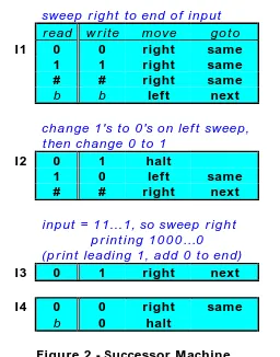
Like programs, Turing machines are designed by coding sequences of instructions. So, let us design and examine an entire machine. The sequence of instructions in figure 2 describes a Turing machine that receives a binary number as input, adds one to it and then halts. Our strategy will be to begin at the lowest order bit (on the right end of the tape) and travel left changing ones to zeros until we reach a zero. This is then changed into a one.

One small problem arises. If the endmarker (#) is reached before a zero, then we have an input of the form 111...11 (the number 2n _{- 1) and must change it to}

1000...00 (or 2n_).

sweep right to end of input

read write move goto

I1 0 0 right same

1 1 right same

# # right same

b b left next

change 1's to 0's on left sweep, then change 0 to 1

I2 0 1 halt

1 0 left same

# # right next

input = 11...1, so sweep right printing 1000…0

(print leading 1, add 0 to end)

I3 0 1 right next

I4 0 0 right same

b 0 halt

Figure 2 - Successor Machine

Have a peek at figure 3. It is a sequence of snapshots of the machine in action. One should note that in the last snapshot (step 9) the machine is not about to execute an instruction. This is because it has halted.

Step 9 ) Step 8 ) Step 7 ) Step 6 ) Step 5 )

I2

I2

I1

I2 I1

Step 2 ) Step 1 ) Start)

Step 3 )

Step 4 ) I1

I1 I1

I1

# 1 0 1 1 . . . # 1 0 1 1 . . .

# 1 0 1 1 . . . # 1 0 1 1 . . .

# 1 0 1 0 . . .

# 1 0 0 0 . . .

# 1 0 1 1 . . .

# 1 0 1 1 . . .

# 1 1 0 0 . . .

# 1 0 1 1 . . .

Figure 3 - Turing Machine Computation

Now that we have seen a Turing machine in action let us note some features, or properties of this class of computational devices.

a) There are no space or time constraints.

b) They may use numbers (or strings) of any size.

c) Their operation is quite simple - they read, write, and move.

For a moment we shall return to the previous machine and discuss its efficiency. If it receives an input consisting only of ones (for example: 111111111), it must:

1) Go to the right end of the input, 2) Return to the left end marker, and 3) Go back to the right end of the input.

This means that it runs for a number of steps more than three times the length of its input. While one might complain that this is fairly slow, the machine does do the job! One might ask if a more efficient machine could be designed to accomplish this task? Try that as an amusing exercise.

Another thing we should note is that when we present the machine with a blank tape it runs for a few steps and gets stuck on instruction I3 where no action is indicated for the configuration it is in since it is reading a blank instead of a zero. Thus it cannot figure out what to do. We say that this in an undefined computation and we shall examine situations such as this quite carefully later.

Up to this point, our discussion of Turing machines has been quite intuitive and informal. This is fine, but if we wish to study them as a model of computation and perhaps even prove a few theorems about them we must be a bit more precise and specify exactly what it is we are discussing. Let us begin.

A Turing machine instruction (we shall just call it an instruction) is a box containing read-write-move-next quadruples. A labeled instruction is an instruction with a label (such as I46) attached to it. Here is the entire machine.

Definition. A Turing machine is a finite sequence of labeled instructions with labels numbered sequentially from I1.

Now we know precisely what Turing machines are. But we have yet to define what they do. Let's begin with pictures and then describe them in our definitions. Steps five and six of our previous computational example (figure 3) were the machine configurations:

I1

# 1 0 1 1 . . .

I2

# 1 0 1 1 . . .

#1011(I1)b... → #101(I2)1b...

This provides the same information as the picture. It is almost as if we took a snapshot of the machine during its computation. Omitting trailing blanks from the description we now have the following computational step

#1011(I1) → #101(I2)1

Note that we shall always assume that there is an arbitrarily long sequence of blanks to the right of any Turing machine configuration.

Definition. A Turing machine configuration is a string of the form x(In)y or x where n is an integer and both x and y are (possibly empty) strings of symbols used by the machine.

So far, so good. Now we need to describe how a machine goes from one configuration to another. This is done, as we all know by applying the instruction mentioned in a configuration to that configuration thus producing another configuration. An example should clear up any problems with the above verbosity. Consider the following instruction.

I17 0 1 right next 1 b right I3

b 1 left same

# # halt

Now, observe how it transforms the following configurations.

a) #1101(I17)01 → #11011(I18)1 b) #110(I17)101 → #110b(I3)01 c) #110100(I17) → #11010(I17)01 d) (I17)#110100 → #110100

Especially note what took place in (c) and (d). Case (c) finds the machine at the beginning of the blank fill at the right end of the tape. So, it jots down a 1 and moves to the left. In (d) the machine reads the endmarker and halts. This is why the instruction disappeared from the configuration.

Definition. For Turing machine configurations C_i and C_j, C_i yields C_j (written C_i → C_j) if and only if applying the instruction in C_i produces C_j .

Definition. If C_i and C_j are Turing machine configurations then C_i

eventually yields C_j (written C_i ⇒ C_j) if and only if there is a finite sequence of configurations C₁ ,C₂ , ... , C_k such that:

C_i = C₁→C₂ → ... →C_{k =} C_{j .}

At the moment we should be fairly at ease with Turing machines and their operation. The concept of computation taking place when a machine goes through a sequence of configurations should also be comfortable.

Let us turn to something quite different. What about configurations which do not yield other configurations? They deserve our attention also. These are called terminal configurations because they terminate a computation). For example, given the instruction:

I3 0 1 halt

1 b right next # # left same

what happens when the machine gets into the following configurations?

a) (I3)#01101 b) #1001(I3)b10 c) #100110(I3) d) #101011

Nothing happens - right? If we examine the configurations and the instruction we find that the machine cannot continue for the following reasons (one for each configuration).

a) The machine moves left and falls off of the tape. b) The machine does not know what to do.

c) Same thing. A trailing blank is being scanned. d) Our machine has halted.

Thus none of those configurations lead to others. Furthermore, any computation or sequence of configurations containing configurations like them must terminate immediately.

We name individual machines so that we know exactly which machine we are discussing at any time. We will often refer to them as M1, M2, M3, or Mi and Mk.

The notation Mi(x) means that Turing machine Mi has been presented with x as

its input. We shall use the name of a machine as the function it computes.

If the Turing machine Mi is presented with x as its input and

eventually halts (after computing for a while) with z written on its tape, we think of Mi as a function whose value is z for the input x.

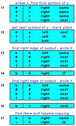
Let us now examine a machine that expects the integers x and y separated by a blank as input. It should have an initial configuration resembling #xby.

erase x, find first symbol of y

I1 # # right same

0 b right same

1 b right same

b b right next

get next symbol of y - mark place

I2 0 ∗∗∗∗ left next

1 ∗∗ left I5

b b halt

find right edge of output - write 0

I3 b b left same

# # right next

0 0 right next

1 1 right next

I4 b 0 right I7

find right edge of output - write 1

I5 b b left same

# # right next

0 0 right next

1 1 right next

I6 b 1 right next

find the ∗∗ and resume copying

I7 b b right same

∗ b right I2

The Turing machine in figure 4 is what we call a selection machine. These receive several numbers (or strings) as input and select one of them as their output. This one computes the function: M(x, y) = y and selects the second of its inputs. This of course generalizes to any number of inputs, but let us not get too carried away.

Looking carefully at this machine, it should be obvious that it:

1) erases x, and

2) copies y next to the endmarker (#).

But, what might happen if either x or y happens to be blank? Figure it out! Also determine exactly how many steps this machine takes to erase x and copy y. (The answer is about n2 _{steps if x and y are each n bits in length.)}

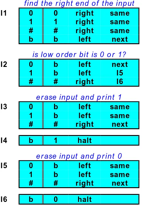
Here is another Turing machine.

find the right end of the input

I1 0 0 right same

1 1 right same

# # right same

b b left next

is low order bit is 0 or 1?

I2 0 b left next

1 b left I5

# # right I6

erase input and print 1

I3 0 b left same

1 b left same

# # right next

I4 b 1 halt

erase input and print 0

I5 0 b left same

1 b left same

# # right next

I6 b 0 halt

It comes from a very important family of functions, one which contains functions that compute relations (or predicates) and membership in sets. These are known as characteristic functions, or 0-1 functions because they only take values of zero and one which denote false and true.

An example is the characteristic function for the set of even integers computed by the Turing machine of figure 5. It may be described:

even(x) =

1 if x is even

0 otherwise 

 



This machine leaves a one upon its tape if the input ended with a zero (thus an even number) and halts with a zero on its tape otherwise (for a blank or odd integers). It should not be difficult to figure out how many steps it takes for an input of length n.

Now for a quick recap and a few more formal definitions. We know that Turing machines compute functions. Also we have agreed that if a machine receives x as an input and halts with z written on its tape, or in our notation:

(I1)#x ⇒ #z

then we say that M(x) = z. When machines never halt (that is: run forever or reach a non-halting terminal configuration) for some input x we claim that the value of M(x) is undefined just as we did with programs. Since output and halting are linked together, we shall precisely define halting.

Definition. A Turing machine halts if and only if it encounters a halt

instruction during computation and diverges otherwise.

So, we have machines that always provide output and some that do upon occasion. Those that always halt compute what we shall denote the total functions while the others merely compute partial functions.

We now relate functions with sets by discussing how Turing machines may characterize the set by deciding which inputs are members of the set and which are not.

Definition. The Turing machine M decides membership in the set A if

and only if for every x, if x ∈ A then M(x) = 1, otherwise M(x) = 0.

at all about elements that were not in the set. Then you could build a machine which halted when given a member of the set and diverged (ran forever or entered a non-halting terminal configuration) otherwise. This is called accepting the set.

Definition. The Turing machine M accepts the set A if and only if for all

x, M(x) halts for x in A and diverges otherwise.

At this point two rather different models or systems of computation have been presented and discussed. One, programs written in the NICE programming language, has a definite computer science flavor, while the other, Turing machines, comes from mathematical logic. Several questions surface.

• which system is better?

• is one system more powerful than the other?

The programming language is of course more comfortable for us to work with and we as computer scientists tend to believe that programs written in similar languages can accomplish any computational task one might wish to perform. Turing machine programs are rather awkward to design and there could be a real question about whether they have the power and flexibility of a modern programming language.

In fact, many questions about Turing machines and their power arise. Can they deal with real numbers? arrays? Can they execute while statements? In order to discover the answers to our questions we shall take what may seem like a rather strange detour and examine the NICE programming language in some detail. We will find that many of the features we hold dear in programming languages are not necessary (convenient, yes, but not necessary) when our aim is only to examine the power of a computing system.

To begin, what about numbers? Do we really need all of the numbers we have in the NICE language? Maybe we could discard half of them.

Negative numbers could be represented as positive numbers in the following manner. If we represent numbers using sign plus absolute value notation, then with companion variables recording the signs of each of our original variables we can keep track of all values that are used in computation. For example, if the variable x is used, we shall introduce another named signx that will have the value 1 if x is positive and 0 if x is negative. For example:

value x signx

19 19 1

Representing numbers in this fashion means that we need not deal with negative numbers any longer. But, we shall need to exercise some caution while doing arithmetic. Employing our new convention for negative numbers, multiplication and division remain much the same although we need to be aware of signs, but addition and subtraction become a bit more complicated. For example, the assignment statement z = x + y becomes the following.

if signx = signy then

begin z = x + y; signz = signx end else if x > y

then begin z = x - y; signz = signx end else begin z = y - x; signz = signy end

This may seem a bit barbaric, but it does get the job done. Furthermore, it allows us to state that we need only nonnegative numbers.

[NB. An interesting side effect of the above algorithm is that we now have two different zeros. Zero can be positive or negative, exactly like some second-generation computers. But this will not effect arithmetic as we shall see.]

Now let us rid ourselves of real or floating point numbers. The standard computer science method is to represent the number as an integer and specify where the decimal point falls. Another companion for each variable (which we shall call pointx) is now needed to specify how many digits lie behind the decimal point. Here are three examples.

value x signx pointx

537 537 1 0

0.0025 25 1 4

-6.723 6723 0 3

Multiplication remains rather straightforward, but if we wish to divide, add, or subtract these numbers we need a scaling routine that will match the decimal points. In order to do this for x and y, we must know which is the greater number. If pointx is greater than pointy we scale y with the following code:

while pointy < pointx do begin

y = y*10;

and then go through the addition routine. Subtraction (x - y) can be accomplished by changing the sign (of y) and adding.

As mentioned above, multiplication is rather simple because it is merely:

z = x*y;

pointz = pointx + pointy;

if signx = signy then signz = 1 else signz = 0;

After scaling, we can formulate division in a similar manner.

Since numbers are never negative, a new sort of subtraction may be introduced. It is called proper subtraction and it is defined as:

x – y = maximum(0, x – y).

Note that the result never goes below zero. This will be useful later.

A quick recap is in order. None of our arithmetic operations lead below zero and our only numbers are the nonnegative integers. If we wish to use negative or real (floating point) numbers, we must now do what folks do at the machine language level; fake them!

Now let's continue with our mutilation of the NICE language and destroy expressions! Boolean expressions are easy to compute in other ways if we think about it. We do not need E₁ > E₂ since it is the same as:

E₁ ≥ E₂ and not E₁ = E₂

Likewise for E₁ < E₂. With proper subtraction, the remaining simple Boolean arithmetic expressions can be formulated arithmetically. Here is a table of substitutions. Be sure to remember that we have changed to proper subtraction and so a small number minus a large one is zero.

E₁ ≤ E₂ E₁ ≥ E₂ E₁ = E₂

E₁ - E₂ = 0 E₂ - E₁ = 0

(E₁ - E₂) + (E₂ - E₁) = 0

these expressions to variables as above and then use those variables in the while or if statements. Only the following two Boolean expressions are needed.

x = 0 not x = 0

Whenever a variable such as z takes on a value greater than zero, the (proper subtraction) expression 1 - z turns its value into zero. Thus Boolean expressions which employ logical connectives may be restated arithmetically. For example, instead of asking if x is not equal to 0 (i.e. not x = 0), we just set z to 1 - x and check to see if z is zero. Thee transformations necessary are included in the chart below and are followed by checking z for zero.

not x = 0

x = 0 and y = 0 x = 0 or y = 0

z = 1 - x z = x + y z = x*y

Using these conversions, Boolean expressions other than those of the form x = 0 are no longer found in our programs.

Compound arithmetic expressions are not necessary either. We shall just break them into sequences of statements that possess one operator per statement. Now we no longer need compound expressions of any kind!

What next? Well, for our finale, let's remove all of the wonderful features from the NICE language that took language designers years and years to develop.

a) Arrays. We merely encode the elements of an array into a simple variable and use this. (This transformation appears as an exercise!)

b) Although while statements are among the most important features of structured programming, a statement such as:

while x = 0 do S

(recall that only x = 0 exists as a Boolean expression now) is just the same computationally as:

10: z = 1 - x;

if z = 0 then goto 20; S;

goto 10

c) The case statement is easily translated into a barbaric sequence of tests and transfers. For example, consider the statement:

case E of: N₁: S₁; N₂: S₂; N₃: S₃ endcase

Suppose we have done some computation and set x, y, and z such that the following statements hold true.

if x = 0 then E = N₁ if y = 0 then E = N₂ if z = 0 then E = N₃

Now the following sequence is equivalent to the original case.

if x = 0 then goto 10; if y = 0 then goto 20; if z = 0 then goto 30; goto 40;

10: begin S1; goto 40 end;

20: begin S2; goto 40 end;

20: begin S3; goto 40 end;

40: (* next statement *)

d) if-then-else and goto statements can be simplified in a manner quite similar to our previous deletion of the case statement. Unconditional transfers (such as goto 10) shall now be a simple if statement with a little preprocessing. For example:

z = 0;

if z = 0 then goto 10;

And, with a little bit of organization we can remove any Boolean expressions except x = 0 from if statements. Also, the else clauses may be discarded after careful substitution.

e) Arithmetic. Let's savage it almost completely! Who needs multiplication when we can compute z = x*y iteratively with:

z = 0;

Likewise addition can be discarded. The statement z = x + y can be replaced by the following.

z = x;

for n = 1 to y do z = z + 1;

The removal of division and subtraction proceeds in much the same way. All that remains of arithmetic is successor (x + 1) and predecessor (x - 1).

While we're at it let us drop simple assignments such as x = y by substituting:

x = 0;

for i = 1 to y do x = x + 1;

f) The for statement. Two steps are necessary to remove this last vestige of civilization from our previously NICE language. In order to compute:

for i = m to n do S

we must initially figure out just how many times S is to be executed. We would like to say that;

t = n - m + 1

but we cannot because we removed subtraction. We must resort to:

z = 0; t = n; t = t + 1; k = m;

10: if k = 0 then goto 20; t = t - 1;

k = k - 1;

if z = 0 then go to 10; 20: i = m;

30: if t = 0 then goto 40; S;

t = t - 1; i = i + 1;

if z = 0 then go to 30; 40: (* next statement *);

Loops involving downto are similar.

Now it is time to pause and summarize what we have done. We have removed most of the structured commands from the NICE language. Our deletion strategy is recorded the table of figure 1. Note that statements and structures used in removing features are not themselves destroyed until later.

Category Item Deleted Items Used

Constants negative numbers

floating point numbers

extra variables case

extra variables while

Boolean arithmetic operations

logical connectives arithmetic

Arrays arrays arithmetic

Repetition while goto, if-then-else Selection case, else if-then

Transfer unconditional goto if-then Arithmetic multiplication

addition division subtraction

simple assignment

addition, for successor, for subtraction, for predecessor, for successor, for, if-then Iteration for If-then, successor,

predecessor

Figure 1 - Language Destruction

In fact, we shall start from scratch. A variable is a string of lower case Roman letters and if x is an arbitrary variable then an (unlabeled) statement takes one of the following forms.

x = 0 x = x + 1 x = x - 1

if x = 0 then goto 10 halt(x)

In order to stifle individuality, we mandate that statements must have labels that are just integers followed by colons and are attached to the left-hand sides of statements. A title is again the original input statement and program heading. As before, it looks like the following.

program name(x, y, z)

Definition. A program consists of a title followed by a sequence of consecutively labeled instructions separated by semicolons.

An example of a program in our new, unimproved SMALL programming language is the following bit of code. We know that it is a program because it conforms to the syntax definitions outlined above. (It does addition, but we do not know this yet since the semantics of our language have not been defined.)

program add(x, y); 1: z = 0

2: if y = 0 then goto 6; 3: x = x + 1;

4: y = y - 1;

5: if z = 0 then go to 2; 6: halt(x)

On to semantics! We must now describe computation or the execution of SMALL programs in the same way that we did for Turing machines. This shall be carried out in an informal manner, but the formal definitions are quite similar to those presented for Turing machine operations in the last section.

Computation, or running SMALL language programs causes the value of variables to change throughout execution. In fact, this is all computation entails. So, during computation we must show what happens to variables and their values. A variable and its value can be represented by the pair:

If at every point during the execution of a program we know the environment, or the contents of memory, we can easily depict a computation. Thus knowing what instruction we are about to execute and the values of all the variables used in the program tells us all we need know at any particular time about the program currently executing.

Very nearly as we did for Turing machines, we define a configuration to be the string such as:

k <x1, v1><x2, v2> ... <xn, vn>

where k is an instruction number (of the instruction about to be executed), and the variable-value pairs show the current values of all variables in the program.

The manner in which one configuration yields another should be rather obvious. One merely applies the instruction mentioned in the configuration to the proper part of the configuration, that is, the variable in the instruction. The only minor bit of defining we need to do is for the halt instruction. As an example, let instruction five be halt(z). Then if x, y, and z are all of the variables in the program, we say that:

5

<

> <

> <

>

Note that a configuration may be either an integer followed by a sequence of variable-value pairs or an integer. Also think about why a configuration is an integer. This happens if and only if a program has halted. We may now reuse the Turing machine system definition for eventually yielding and computation has almost been completely defined.

Initially the following takes place when a SMALL program is executed.

a) input variables are set to their input values b) all other variables are set to zero

c) execution begins with instruction number one

From this we know what an initial configuration looks like.

Halting configurations were defined above to be merely numbers. Terminal configurations are defined in a manner almost exactly the same as for Turing machines. We recall that this indicates that terminal configurations might involve undefined variables and non-existent instructions.

We will now claim that programs compute functions and that all of the remaining definitions are merely those we used in the section about Turing machines. The formal statements of this is left as an exercise.

At this point we should believe that any program written in the NICE language can be rewritten as a SMALL program. After all, we went through a lot of work to produce the SMALL language! This leads to a characterization of the computable functions.

Our discussion of what comprises computation and how exactly it takes place spawned three models of computation. There were two programming languages (the NICE language and the SMALL language) and Turing Machines. These came from the areas of mathematical logic and computer programming.

It might be very interesting to know if any relationships between three systems of computation exist and if so, what exactly they are. An obvious first question to ask is whether they allow us to compute the same things. If so, then we can use any of our three systems when demonstrating properties of computation and know that the results hold for the other two. This would be rather helpful.

First though, we must define exactly what we mean by equivalent programs and equivalent models of computation. We recall that both machines and programs compute functions and then state the following.

Definition. Two programs (or machines) are equivalent if and only if they compute exactly the same function.

Definition. Two models of computation are equivalent if and only if the same exact groups of functions can be computed in both systems.

Let us look a bit more at these rather official and precise statements. How do we show that two systems permit computation of exactly the same functions? If we were to show that Turing Machines are equivalent to NICE programs, we should have to demonstrate:

• For each NICE program there is an equivalent Turing machine

• For each Turing machine there is an equivalent NICE program

This means that we must prove that for each machine M there is a program P such that for all inputs x: M(x) = P(x) and vice versa.

An fairly straightforward equivalence occurs as a consequence of the language destruction work we performed in painful detail earlier. We claim that our two languages compute exactly the same functions and shall provide an argument for this claim in the proof of theorem 1.

Theorem 1. The following classes of functions are equivalent:

a) the computable functions,

b) functions computable by NICE programs, and c) functions computable by SMALL programs.

Informal Proof. We know that the classes of computable functions and those computed by SMALL programs are identical because we defined them to be the same. Thus by definition, we know that:

computable = SMALL.

The next part is almost as easy. If we take a SMALL program and place begin and end block delimiters around it, we have a NICE program since all SMALL instructions are NICE too (in technical terms). This new program still computes exactly the same function in exactly the same manner. This allows us to state that:

computable = SMALL ⊂ NICE.⊂

Our last task is not so trivial. We must show that for every NICE program, there is an equivalent SMALL program. This will be done in an informal but hopefully believable manner based upon the section on language destruction.

Suppose we had some arbitrary NICE program and went through the step-by-step transformations upon the statements of this program that turn it into a SMALL program. If we have faith in our constructions, the new SMALL program computes exactly same function as the original NICE program. Thus we have shown that

computable = SMALL = NICE

and this completes the proof.

That was really not so bad. Our next step will be a little more involved. We must now show that Turing machines are equivalent to programs. The strategy will be to show that SMALL programs can be converted into equivalent Turing machines and that Turing machines in turn can be transformed into equivalent NICE programs. That will give us the relationship:

This relationship completes the equivalence we wish to show when put together with the equivalence of NICE and SMALL programs shown in the last theorem. Let us begin by transforming SMALL programs to Turing machines.

Taking an arbitrary SMALL program, we first reorganize it by renaming the variables. The new variables will be named x₁, x₂, ... with the input variables leading the list. An example of this is provided in figure 1.

program example(x, y) program example(x1, x2)

1: w = 0; 1: x3 = 0;

2: x = x + 1; 2: x1 = x1 + 1;

3: y = y - 1; 3: x2 = x2 - 1;

4: if y = 0 then goto 6; 4: if x2 = 0 then goto 6;

5: if w = 0 then goto 2; 5: if x3 = 0 then goto 2;

6: halt(x) 6: halt(x1)

Figure 1 - Variable Renaming

Now we need to design a Turing machine that is equivalent to the SMALL program. The variables used in the program are stored on segments of the machine’s tape. For the above example with three variables, the machine should have a tape that looks like the one shown below.

# x1 x2 x3 . . .

Note that each variable occupies a sequence of squares and that variables are separated by blank squares. If x₁ = 1101 and x₂ = 101 at the start of computation, then the machine needs to set x₃ to zero and create a tape like:

0 1

# 1 1 1 0 1 0 . . .

Now what remains is to design a Turing machine which will mimic the steps taken by the program and thus compute exactly the same function as the program in as close to the same manner as possible.

For this machine design we shall move to a general framework and consider what happens when we transform any SMALL program into a Turing machine.

Set up the Tape Program Instruction 1 Program Instruction 2

• •• •

Program Instruction m

Figure 2 - SMALL Program Simulator

Each of the m+1 sections of the Turing machine in figure 2 contains several Turing machine instructions. Let us examine these sections.

Setting up the tape is not difficult. If the program uses x₁, ... x_n as variables and the first k are input parameters, then the tape arrives with the values of the first k variables written upon it in the proper format. Now space for the remaining variables (x_k+1 through x_n) must be added to the end of the input section. To begin, we must go one tape square past the end of x_k. Since two adjacent blanks appear at the end of the input, the following instruction pair finds the square where x_k+1 should be written.

# # right same 0 0 right same 1 1 right same b b right next

0 0 right previous 1 1 right previous

b b left next

Now that the tape head is on the blank following x_k we need to initialize the remaining variables (x_k+1, ... , x_n). This is easily done by n-k instruction pairs exactly like the following.

b 0 right next

b b right next

Here is the general format for executing a SMALL program instruction.

a) Find the variable used in the program instruction

b) Modify it according to the program instruction

c) Prepare to execute the next instruction

In the following translation examples, we note that there is only one variable in each instruction. We shall assume that the instruction we are translating contains the variable named x_i.

To locate the variable x_i, we first move the tape head to the first character of x₁ by going all the way to the left endmarker and moving one tape square to the right with the instruction:

0 0 left same 1 1 left same

b b left same

# # right next

At this point we use i-1 instructions of the form:

0 0 right same 1 1 right same b b right next

to move right past the variables x₁, ... , x_i-1 and place the tape head on the first character of x_i. Now we are ready to actually execute the instruction.

We shall now examine the instructions of the SMALL language one at a time and show how to execute them on a Turing machine. Recall that we begin execution with the tape head on the first character of the variable (x_i) mentioned in the program instruction.

a) The Turing machine executes x_i = 0 by changing the characters of x_i to zero with the instruction:

0 0 right same 1 0 right same b b right next

If x_i is zero then nothing must be changed since in the SMALL language there are no numbers less than zero. Recall that we use proper subtraction. One way to prevent this is to first modify the program so that we only subtract when x_i is greater than zero. Whenever we find subtraction, just insert a conditional instruction like this:

74: if xi = 0 then goto 76;

75: xi = xi - 1;

76:

Here is the pair of Turing machine instructions that accomplish proper predecessor .

move to the right end of x_i

0 0 right same 1 1 right same b b left next

go back, flipping the bits

0 1 left same 1 0 left next

c) We designed a machine for x_i = x_i + 1 as our first Turing machine example. This machine will not work properly if x_i is composed totally of ones though since we need to expand the space for x_i one square in that case. For example if the portion of tape containing x_i resembles this:

0 1

. . . _{1 1 1 1 1 1 0} . . .

then adding one changes it to:

. . . _{0 1 1 0 0 0 0 1 1 0} . . .

Thus we need to move the variables x_i+1, ... , x_n to the right one square before adding one to x_i. This is left as an exercise.

Otherwise control must be transferred to the next program instruction. If I64 is the Turing machine instruction that begins the section for the execution of program instruction 10 then the correct actions are accomplished by the following instruction.

0 0 right same 1 1 right next b b right I64

e) The selector machine seen earlier computed the function f(x, y) = y. The halt(x_i) instruction is merely the more general f(x₁, ... , x_n) = x_i.

We have defined a construction method that will change a SMALL program into a Turing machine. We need now to show that the program and the machine are indeed equivalent, that is, they compute exactly the same functions for all possible inputs. We shall do this by comparing configurations in another informal argument.

Recalling our definitions of Turing machine configurations and program configurations, we now claim that if a program enters a configuration of the form:

k <x₁, v₁> <x₂, v₂> ... <x_n, v_n>

(where the k-th instruction in the program refers to the variable x_i) then the Turing machine built from the program by the above construction will eventually enter an equivalent configuration of the form:

#v₁bv₂b ... (Im)v_ib ... bv_n

Where Im is the Turing machine instruction at the beginning of the set of instructions that perform program instruction k. In other words, the machine and the program go through equivalent configurations. And, if the program's entire computation may be represented as:

1 <x₁, v₁> ... <x_k, v_k> <x_k+1, 0> ... <x_k, 0> ⇒ z then the Turing machine will perform the computation:

(I1)#v₁b ... bv_k ⇒ #z

Theorem 2. For every SMALL program there is a Turing machine which

computes exactly the same function.

An interesting question about our translation of programs into Turing machines involves complexity. The previous transformation changed a SMALL program into a larger Turing machine and it is obvious that the machine runs for a longer period of time than the program. An intellectually curious reader might work out just what the relationship between the execution times might be.

The last step in establishing the equivalence of our three models of computation is to show that NICE programs are at least as powerful as Turing machines. This also will be carried out by a construction, in this case, one that transforms Turing machines into programs.

First we need a data structure. The Turing machine's tape will be represented as an array of integers. Each element of the array (named tape of course) will have the contents of a tape square as its value. Thus tape[54] will contain the symbol from the Turing machine's alphabet that is written on the tape square which is 54th _{from the left end of the tape. In order to cover Turing machine}

alphabets of any size we shall encode machine symbols. The following chart provides an encoding for our standard binary alphabet, but it extends easily to any size alphabet.

TM symbol b 0 1 #

tape[i] 0 1 2 3

If a Turing machine's tape contains:

0 1

# 1 1 . . .

then the program’s array named tape would contain:

tape = <3, 2, 2, 1, 2, 0, 0, ... >

Thinking ahead just a little bit, what we are about to do is formulate a general method for translating Turing machines into programs that simulate Turing machines. Two indexing variables shall prove useful during our simulation. One is named head and its value denotes the tape square being read by the machine. The other is called instr and its value provides the number of the Turing machine instruction about to be executed.

move go to

left head = head - 1 I43 instr = 43 right head = head + 1 same

next instr = instr + 1

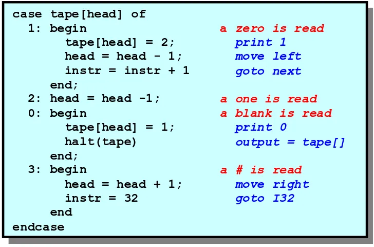
It should be almost obvious how we shall program a Turing machine instruction. For example, the instruction:

0 1 left next 1 1 left same

b 0 halt

# # right I32

is programmed quite easily and elegantly in figure 3.

case tape[head] of

1: begin a zero is read tape[head] = 2; print 1

head = head - 1; move left

instr = instr + 1 goto next

end;

2: head = head -1; a one is read

0: begin a blank is read

tape[head] = 1; print 0

halt(tape) output = tape[]

end;

3: begin a # is read

head = head + 1; move right

instr = 32 goto I32

end endcase

Figure 3 - Translating a Turing Machine Instruction

case instr of

1: case tape[head] of 2: case tape[head] of

• • •

n: case tape[head] of endcase

Figure 4 - All of a Turing Machine’s Instructions

Since a Turing machine starts operation on its first square and begins execution with its first instruction, we must set the variables named head and instr to one at the beginning of computation. Then we just run the machine until it encounters a halt, tries to leave the left end of the tape, or attempts to do something that is not defined. Thus a complete Turing machine simulation program is the instruction sequence surrounded by a while that states:

‘while the Turing machine keeps reading tape squares do …’

and resembles that of figure 5.

program name(tape);

var instr, head: integer; tape[]: array of integer;

begin

instr = 1; head = 1 while head > 0 do case instr of

• • •

endcase end

Figure 5 - Simulation of a Turing Machine

This completes the transformation.

Theorem 3. Every function that is Turing machine computable can also

be computed by a NICE program.

What we have done in the last two sections is show that we can transform programs and machines. The diagram below illustrates these transformations.

NICE

TM

SMALL

The circularity of these transformations shows us that we can go from any computational model to any other. This now provides the proof for our major result on system equivalence.

Theorem 4. The class of computable functions is exactly the class of

functions computed by either Turing machines, SMALL programs, or NICE programs

This result is very nice for two major reasons. First, it reveals that two very different concepts about computability turn out to be identical in a sense. This is possibly surprising. And secondly, whenever in the future we wish to demonstrate some property of the computable functions, we have a choice of using machines or programs. We shall use this power frequently in our study of the nature of computation.

Our examination of the equivalence of programs and machines brought us more than just three characterizations of the computable functions. In fact, a very interesting byproduct is that the proof of theorem 3 can be used to show a feature of the NICE language that programming language researchers find important, if not essential.

Corollary. Every NICE program may be rewritten so that it contains no

goto statements and only one while statement.

Proof Sketch. In order to remove goto's and extra loops from NICE programs, do the following. Take any NICE program and:

a) Convert it to a SMALL program. b) Change this into a Turing machine.

c) Translate the machine into a NICE program.

The previous results in this section provide the transformations necessary to do this. And, if we examine the final construction from machines to NICE programs, we note that the final program does indeed meet the required criteria.

We know now that Turing machines and programming languages are equivalent. Also, we have agreed that they can be used to compute all of the things that we are able to compute. Nevertheless, maybe there is more that we can discover about the limits of computation.

With our knowledge of computer science, we all would probably agree that not too much can be added to programming languages that cannot be emulated in either the NICE or the SMALL language. But possibly a more powerful machine could be invented. Perhaps we could add some features to the rather restricted Turing machine model and gain computing power. This very endeavor claimed the attention of logicians for a period of time. We shall now review some of the more popular historical attempts to build a better Turing machine.

Let us begin by correcting one of the most unappetizing features of Turing machines, namely the linear nature of their tapes. Suppose we had a work surface resembling a pad of graph paper to work upon? If we wished to add two numbers it would be nice to be able to begin by writing them one above the other like the following.

#

1 1

1 0

1 1

0

1

. . .

. . .

. . .

Then we can add them together in exactly the manner that we utilize when working with pencil and paper. Sweeping the tape from right to left, adding as we go, we produce a tape like that below with the answer at the bottom.

#

1 1

1 0

1 1

0

1

. . .

. . .

. . .

1 1

1 0

0

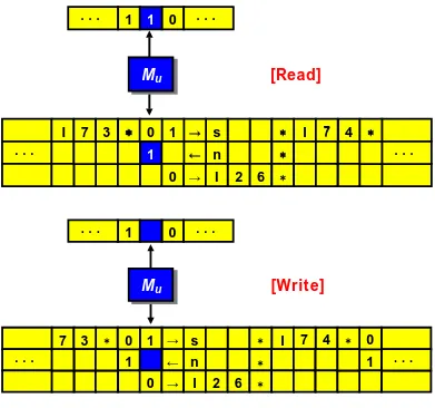
reading and writing single symbols, the machine reads and writes columns of symbols.

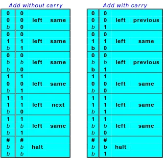
The 3-track addition process shown above could be carried out as follows. First, place the tape head at the right end of the input. Now execute the pair of instructions pictured in figure 1 on a sweep to left adding the two numbers together.

Add without carry Add with carry

0 0 0 0

0 0 left same 0 0 left previous

b 0 b 1

0 0 0 0

1 1 left same 1 1 left same

b 1 b 0

0 0 0 0

b b left same b b left previous

b 0 b 1

1 1 1 1

0 0 left same 0 0 left same

b 1 b 0

1 1 1 1

1 1 left next 1 1 left same

b 0 b 1

1 1 1 1

b b left same b b left same

b 1 b 0

# # # #

b b halt b b halt

b b b 1

Figure 1 - Addition using Three Tracks

Comparing this 3-track machine with a 1-track machine designed to add two numbers, it is obvious that the 3-track machine is:

• easier to design, • more intuitive, and • far faster

Theorem 1. The class of functions computed by n-track Turing machines is the class of computable functions.

Proof Sketch. Since n-track machines can do everything that 1-track machines can do, we know immediately that every computable function can be computed by an n-track Turing machine. We must now show that for every n-track machine there is an equivalent 1-track machine.

We shall demonstrate the result for a specific number of tracks since concrete examples are always easier to formulate and understand than the general case. So, rather than show this result for all values of n at once, we shall validate it for 2-track machines and claim that extending the result to any number of tracks is an fairly simple expansion of our construction.

Our strategy is to encode columns of symbols as individual symbols. For two-track machines using zero, one and blank we might use the following encoding of pairs into single symbols.

0 1 b 0 1 b 0 1 b

column

0 0 0 1 1 1 b b b

code u v w x y z 0 1 b

The encoding transforms 2-track tapes into 1-track tapes. Here is a simple example.

0

1 1

0

0

1 0

0

. . .

. . .

u

v

x

0

z

. . .

Now all that is needed is to translate the instructions for a 2-track machine into equivalent instructions for the 1-track machine that uses the encoding. For example, the 2-track machine instruction below may be replaced by that for a 1-track machine to the right.

0 1

0 0 right next u v right next

1 1 ! v y left same

0 1 left same b 0 halt

b 0

To finish the proof, we argue that if the original 2-track machine were run side-by-side with the new 1-track machine their computations would look identical after taking the tape encoding into account.

That takes care of the actual computation. However, we neglected to discuss input and output conventions. Input is simple, we merely assume that the 1-track machine begins computation with the 2-track input encoding upon the ta