Maxwell Boltzmann Distribution in Solids

(1)

http://www.scirp.org/journal/jamp ISSN Online: 2327-4379 ISSN Print: 2327-4352

DOI: 10.4236/jamp.2018.63052 Mar. 28, 2018 602 Journal of Applied Mathematics and Physics

Maxwell-Boltzmann Distribution in Solids

Pirooz Mohazzabi, Siva P. Shankar

Department of Mathematics and Physics, University of Wisconsin-Parkside, Kenosha, WI, USA

Abstract

The velocity distribution functions of particles in one- and three-dimensional harmonic solids are investigated through molecular dynamics simulations. It is shown that, as in the case of dense fluids, these distribution functions still obey the Maxwell-Boltzmann law and the assumption of molecular chaos re-mains valid even at low temperatures.

Keywords

Maxwell-Boltzmann, Velocity, Distribution Function, Solids

1. Introduction

In the classical theory of ideal gases, the velocity distribution function is derived from the Boltzmann transport equation based on the assumption of molecular chaos and a dilute enough gas so that ternary and higher collisions can be ig-nored [1]. In an ideal gas trajectories of the particles are straight lines, meaning that the particles interact through short range potentials, such as hard-sphere or Lennard-Jones potentials. Under these conditions, the velocity distribution of the particles is described by the Maxwell-Boltzmann distribution function.

However, it can be shown that the Maxwell-Boltzmann distribution function describes molecular velocities even in non-ideal gases [2] [3], even in the presence of long-range interactions between the particles of the system such as Coulomb potential, as long as the assumption of molecular chaos remains valid [4]. Not long ago, extremely dense fluid systems with strong interactions between its par-ticles were investigated through molecular dynamics simulations. It was shown that even in these systems the velocity distribution of the particles is Maxwellian and the assumption of molecular chaos remains valid [4].

In what follows, we extend this investigation to include solids with strong harmonic interactions between its particles. Solids are interesting because con-trary to fluids where the particles can move throughout the entire volume avail-How to cite this paper: Mohazzabi, P. and

Shankar, S.P. (2018) Maxwell-Boltzmann Distribution in Solids. Journal of Applied Mathematics and Physics, 6, 602-612. https://doi.org/10.4236/jamp.2018.63052

Received: February 13, 2018 Accepted: March 25, 2018 Published: March 28, 2018

(2)

DOI: 10.4236/jamp.2018.63052 603 Journal of Applied Mathematics and Physics able to the fluid, in solids the particles can only oscillate about their mean equi-librium positions, and for strong interactions these oscillations are restricted to a very limited region of space.

The choice of harmonic interactions between the particles is due to the fact that any interaction between particles of a solid can be approximated by a har-monic potential as long as the displacements of the particles from their equili-brium positions remain small. Of course, solids with harmonic interatomic in-teractions have long been studied extensively [5]-[11]. However, to the best of the author’s knowledge, velocity distribution of atoms in these solids, which is the subject of this investigation, has not been discussed or reported in the litera-ture.

2. Theoretical Background

The normalized Maxwell-Boltzmann velocity distribution function (or probabil-ity densprobabil-ity function) of a perfect gas in one dimension is given by [12]

( )

1 2exp 2

2π 2 x x mv m f v kT kT     =_ _ _− _

   .(1)

Assuming molecular chaos, the velocity distribution function in three dimen-sions can be written as the product of the one-dimensional distribution func-tions [1] [4],

(

, ,

)

( )

3 2exp 2

2π 2

x y z x y z

m mv

f v v v f v f v f v

kT kT

 

= =_ _ _− _

   

(2)

where 2 2 2 2

x y z

v =v +v +v . Then the probability of finding a particle with velocity in

the interval

(

v v vx, y, z

)

to

(

vx+d ,v vx y+d ,v vy z+dvz

)

is f v v v

(

x, y, z

)

d d dv v vx y z.

Transforming this probability to spherical coordinates in velocity space with

2

d d dv v vx y z =v vd sin d d

θ θ φ

and integrating over θ and φ, we obtain the Max-well-Boltzmann speed distribution function in three dimensions,

( )

4π 3 2 2 2

exp

2π 2

m mv

f v v

kT kT

 

= _ _ _− _

   .

(3)

As stated above, in this work we assume a harmonic potential for interaction of the atoms. This is because any general interatomic potential energy function of two atoms can be expanded is a Taylor series about the equilibrium position of the atoms,

( )

( )(

)

( )(

)

2

0 0 0 0 0

1 1

1! 2!

u r =u r + u r′ r−r + u r′′ r−r +

(4) where r is the distance between the two atoms and r0 is the equilibrium distance.

The first term on the right hand side is a constant, which defines the reference of the potential energy. This constant can arbitrarily be set equal to zero. The second term is zero because the force on the particle is given by

(3)

DOI: 10.4236/jamp.2018.63052 604 Journal of Applied Mathematics and Physics and at equilibrium the force on the particle is zero. The coefficient of the third term is positive because the potential energy is a minimum at a stable brium point. Finally, for small displacements of the particles from their equili-brium (r−r0), we can ignore the higher-order terms in the expansion (4), and

write

( )

(

)

2 0

1 2

u r = c r−r

(6) where c=u r′′

( )

0 is a positive constant. Therefore, for small deviations from

equilibrium, a particle under any interatomic potential energy function in a solid experiences a harmonic potential. However, it should be pointed out that this analysis is valid as long as the potential energy function is not intrinsically non-linear [13].

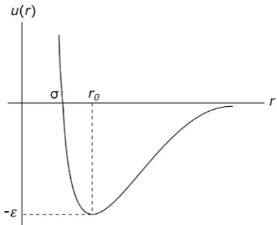
The interactions between atoms in many simple solids are described by Len-nard-Jones (6-12) potential energy function [14] [15] [16],

( )

4 12 6

u r

r r

σ σ

_{ } _{ }  = _{ } −_{ } 

   

 

 



(7)

where  and σ are constants with units of energy and length, respectively. The first term in this equation corresponds to attraction between the two atoms resulting from van der Waals interaction between them [14]. The second term corresponds to repulsion arising from overlap of the electron distributions of the atoms and the Pauli Exclusion Principle. This term becomes dominant at small distances between the atoms. The meaning of the constants  and σ in Equation (7) can be inferred from Figure 1, which schematically shows the graph of Lennard-Jones potential energy function. The minimum of the po-tential energy − corresponds to the equilibrium distance between two atoms

0 r.

Differentiating Equation (7) with respect to r and setting it equal to zero gives

1 6

0 2

r = σ. ₍₈₎

[image:3.595.272.472.542.704.2]

A second differentiation of Equation (7) and its evaluation at r=r0 gives

(4)

DOI: 10.4236/jamp.2018.63052 605 Journal of Applied Mathematics and Physics

( )

0

2

0 2 1 3 2

d 72

d 2

r r u r

u r

r ₌ σ

′′ = =  .

(9)

Therefore according to Equation (6), for small deviations from equilibrium, the Lennard-Jones potential reduces to a harmonic potential given by

( )

(

)

2

0 1 3 2 1 72 2 2

u r r r

σ   = _ _ −    _. (10)

3. Molecular Dynamics Simulations

We investigate both a one-dimensional and a three-dimensional solid. This is because in some cases one-dimensional systems behave differently from those of higher dimensions. In addition, correlating the results of the one-dimensional system with those of the three-dimensional system can further verify the validity of the assumption of molecular chaos. Furthermore, in order to mimic an actual atomic solid in our simulations, we consider argon-like particles interacting ac-cording to a harmonic potential energy function given by Equation (10).

Since the actual atomic parameters are very small in SI units, we use a reduced system of units. In this system the mass of the atoms m is the unit of mass and the equilibrium distance between the atoms r0 is the unit of length. For argon,

the atomic mass and the Lennard-Jones potential parameters are [15] [17],

26 10 21

6.69 10 kg, 3.42 10 m, 1.65 10 J

m= × − σ = × − = × − . (11)

Therefore, in our system of units, the unit of mass is 26

6.69 10× − kg and the unit of length (r0) is 3.84 10× −10m. Finally, we take =1.65 10× −21J and

120 K

k=

 to be our units of energy and temperature, respectively, where

23 1.38 10 J K

k= × − is the Boltzmann’s constant. This completes our system of

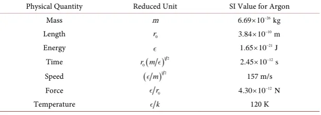
units. Any other physical quantity in our simulations can be written as a combi-nation of these units, as shown in Table 1.

All of the simulations, in one and in three dimensions, were carried out using the velocity form of the Verlet algorithm [18] [19],

( )

(

)

2 1 1 1 1 2 1 2

n n n n

v t a t

v v a a t

ξ+ ξ

[image:4.595.209.540.608.727.2]

+ +  ₌ _{+ ∆ +} _∆    ₌ ₊ ₊ _∆  (12)

Table 1. The system of units used in the molecular dynamics simulations in this work.

Physical Quantity Reduced Unit SI Value for Argon

Mass m 26

6.69 10× − kg

Length r0

10

3.84 10× − m

Energy  21

1.65 10× − J

Time ( )1 2

0

r m 12

2.45 10× − s

Speed ( )1 2

m

 157 m/s

Force r0

12

4.30 10× − N

(5)

DOI: 10.4236/jamp.2018.63052 606 Journal of Applied Mathematics and Physics with a time step of

∆ =

t

0.01

reduced unit, where ξ stands for x, y, or z, and v and a are the corresponding velocity and acceleration, respectively. Furthermore, throughout the investigation periodic boundary conditions were used to reduce the size effect of the systems.

3.1. One-Dimensional Solid

We studied a linear chain of 200 argon-like particles, each of mass m, with spring-like interaction between the adjacent particles,

(

0

)

F= −c r−r ₍₁₃₎

where r is the instantaneous distance between two adjacent atoms and r0 is the

relaxed length of the spring. Since

d

u F

r

= −

(14) according to Equation (10) the constant c in Equation (13) is given by

1 3 2

72 2

c

σ

= 

(15) which, in our reduced system of units, has a value of 72.

The particles were initially arranged on a straight line at one unit of length in-tervals. Each particle was then randomly given a velocity of +1 or −1 reduced unit and then the center of mass of the system was brought to rest. The temper-ature of the system was calculated from

1 2

K = kT

(16) where K is the mean kinetic energy of the particles. The velocity of each

par-ticle was then re-scaled according to the following equation to adjust the tem-perature of the system to the desired value [20],

new d i i

a

T

v v

T

=

(17) where Ta is the actual temperature calculated from (16) and Td is the desired

temperature.

The simulation was allowed to run for 1000 time steps to thermalize the sys-tem before any data were collected. After thermalization, data were collected on the temperature of the system as a function of time step and the velocity distri-bution of the particles over the next 105_{time steps. We also monitored the}

veloc-ity of the center of mass of the system to ensure the center of mass did not drift during the simulation, or there was no “wind” in the system.

We simulated the system with temperatures of

T

=

0.5

and

T

=

1.0

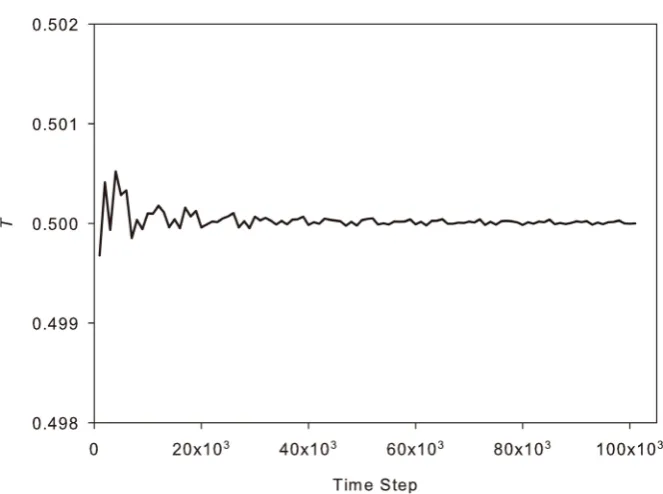
re-duced unit. Figure 2 shows the temperature of the system as a function of time step for

T

=

0.5

reduced unit. As can be seen from this figure, the temperature of the system remained very steady throughout the simulation. The results for

1.0

(6)

[image:6.595.208.540.62.309.2]

Figure 2. Evolution of temperature as a function of time step in the one-dimensional

[image:6.595.210.541.350.595.2]

si-mulation.

Figure 3. Velocity distribution functions for a one-dimensional chain of particles

inte-racting according to a harmonic potential at two different temperatures. The markers are the simulation results and the solid curves are predictions from the Maxwell-Boltzmann distribution law.

(7)

DOI: 10.4236/jamp.2018.63052 608 Journal of Applied Mathematics and Physics corresponding quantities in reduced units. Thus, for

T

=

0.5

,

( )

1 2 e π

v

f v = −

(18) and for

T

=

1.0

,

( )

1 2₂ e 2π

v

f v = − .

(19) These are shown as solid curves in Figure 3. As can be seen, the simulation re-sults are in excellent agreement with the Maxwell-Boltzmann distribution func-tion for molecular velocities.

3.2. Three-Dimensional Solid

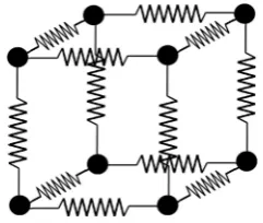
In this part of the investigation, we studies a system of 512 argon-like particles (

8 8 8

× ×

) on a simple cubic lattice, the unit cell of which is shown in Figure 4. Each particle interacted harmonically with its 6 nearest neighbors according to Equation (13) with the same potential parameters described above. As in the one-dimensional case, periodic boundary conditions were used to reduce the size effect of the system.

Each particle was initially given a random velocity in the interval

(

−1,1

)

in each coordinate direction. These velocities were then reduced to bring the center of mass of the system to rest. The temperature of the system was then calculated from

3 2

K = kT

(20) as before, then the velocity components of each particle were re-scaled according to Equation (17) to adjust the temperature of the system to the desired value. The system was allowed to thermalize for 5000 time steps. Then data were col-lected during the next 105_{time steps on temperature and speed distribution of}

the particles for

T

=

0.5

and

T

=

1.0

reduced unit.

Figure 5 shows the temperature of the system as a function of time step for

0.5

[image:7.595.313.434.594.696.2]

T

=

reduced unit. As can be seen from the figure, similar to the one-dimensional case, the temperature of the system remained very uniform throughout the simula-tion. The result for

T

=

1.0

was similar and very uniform.

Figure 6 shows the speed distribution functions obtained in the simulation of

Figure 4. The unit cell of the three-dimensional solid investigated. Each particle interacts

(8)

[image:8.595.208.541.63.308.2]

Figure 5. Evolution of temperature as a function of time step in the three-dimensional

simulation.

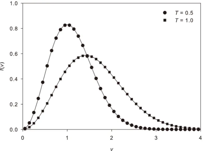
Figure 6. Speed distribution functions for a three-dimensional system of 512 particles

in-teracting according to a harmonic potential at two different temperatures. The markers are the molecular dynamics simulation results and the solid curves are predictions from the Maxwell-Boltzmann distribution law.

[image:8.595.209.542.348.595.2]

(9)

DOI: 10.4236/jamp.2018.63052 610 Journal of Applied Mathematics and Physics respectively

( )

4 ₂ 2 e π

v

f v = v −

(21) and

( )

2 ₂ 2₂ e π

v

f v = v − .

(22) These are shown by solid curves in Figure 6. Again as in the one-dimensional case, the agreement between the molecular dynamics simulations and the Max-well-Boltzmann distribution functions are excellent.

We also point out that in the three-dimensional case as well, each of the veloc-ity distribution functions f v

( )

x , f v

( )

y , f v

( )

z were similar to that of the

one-dimensional system shown in Figure 3, and they were all in near perfect agreement with the one-dimensional Maxwell-Boltzmann distribution function (1).

4. Discussion and Conclusions

Figure 2 and Figure 5 show that during the entire simulation in one- and three-dimensional systems the temperature remained very stable. The large fluctuation at the beginning of the run in each case is due to small number of time steps used in the averaging process.

As pointed out earlier, the Maxwell-Boltzmann velocity distribution function, which was originally obtained for an ideal gas, remains valid even in non-ideal gases and in the presence of long-range interactions between the particles of the system as long as the assumption of molecular chaos remains valid. Later, mole-cular dynamics simulations showed that even in extremely dense fluid systems with strong interactions between its particles velocity distribution of the particles is Maxwellian and the assumption of molecular chaos remains valid.

In this study we have taken the investigation one step further to include solid systems where, contrary to fluid systems, motion of the particles is very limited in space, especially at low temperatures. For the argon-like particles studied, ac-cording to Table 1, the temperatures

T

=

0.5

and

T

=

1.0

reduced unit trans-late into 60 K and 120 K, respectively, which are quite low. At these low temper-atures, the amplitude of the oscillations of the particles is very small and the par-ticles remain in a very limited region of space. In fact, in all of our simulations, the mean deviation of the interatomic distance from its equilibrium value was only about 9% or less across the board. Nevertheless, the results clearly show that even in this case the velocity distribution of the particles remains Maxwel-lian.

(10)

DOI: 10.4236/jamp.2018.63052 611 Journal of Applied Mathematics and Physics in solids, even at low temperatures.

In addition, the Maxwell-Boltzmann distribution function is obtained from the Boltzmann transport equation which, in turn, is based on the assumption of a dilute gas [1]. According to this derivation, therefore, the system must be in the classical regime,

1

Q

n

n  (23)

where n is the particle density and

3 2

2 2π

Q

mkT n

h

 

= _ _

(24) is the quantum concentration of the system [21] [22]. In this equation

34 6.626 10 J s

h= × − ⋅ is the Plank’s constant, which in our reduced system of

units has a value of 0.164 and unit of

( )

1 2 0

r m . For our three-dimensional

sys-tem with simple cubic structure, there is one atom per unit cell and each side of the unit cell has a length r0, therefore, n=N V =1r03. Then with

T

=

0.5

re-duced units, we have

(

)

(

)

(

)

3 2 3 2

3 2 2 2

2

4 3

0

0.164 0.164

1

8 10 1

2π 2π 0.5 π

Q

n N h

n V mkT r mk k

−

   

 

= _ _ =   =  = ×

   

  _  _ _ _  (25)

Therefore, even though the system that we have investigated is a solid at low temperatures, it is still in the classical regime.

References

[1] Huang, K. (1987) Statistical Mechanics. 2nd Edition. Wiley, New York, 60-62, 75-77.

[2] Hirschfelder, J.O., Curtiss, C.F. and Bird, R.B. (1954) Molecular Theory of Gases and Liquids. Wiley, New York, 101.

[3] McQuarrie, D.A. (1976) Statistical Mechanics. Harper & Row, New York, 125. [4] Mohazzabi, P., Helvey, S.L. and McCumber, J. (2002) Maxwellian Distribution in

Non-Classical Regime. Physica A, 316, 314-322.

https://doi.org/10.1016/S0378-4371(02)01020-8

[5] Kittel, C. (1996) Introduction to Solid State Physics. 7th Edition, Wiley, New York, 99.

[6] Rosenberg, H.M. (1978) The Solid State. 2nd Edition, Oxford University Press, Ox-ford, 78-82.

[7] Cochran, W. (1973) The Dynamics of Atoms in Crystals. Edward Arnold Limited, Great Britain, 28.

[8] Wannier, G.H. (1987) Statistical Physics. Dover, New York, 78. [9] Mandl, F. (1988) Statistical Physics. 2nd Edition, Wiley, New York, 150.

[10] Wee, L. and Dhar, A. (2005) Heat Conduction in a Two-Dimensional Harmonic Crystal with Disorder. Physical Review Letters, 95, Article ID: 094302.

(11)

DOI: 10.4236/jamp.2018.63052 612 Journal of Applied Mathematics and Physics https://doi.org/10.1007/BF01614132

[12] Atkins, P.W. (1986) Physical Chemistry. 3rd Edition, W. H. Freeman and Compa-ny, New York, 647-649.

[13] Mohazzabi, P. (2004) Theory and Examples of Intrinsically Nonlinear Oscillators.

American Journal of Physics, 72, 492-498. https://doi.org/10.1119/1.1624114

[14] Kittel, C. (1996) Introduction to Solid State Physics. 7th Edition, Wiley, New York, 55-66.

[15] White, J.A. (1999) Lennard-Jones as a Model for Argon and Test of Extended Re-normalization Group Calculations. Journal of Chemical Physics, 111, 9352-9356.

https://doi.org/10.1063/1.479848

[16] Talu, O. and Myers, A.L. (2001) Reference Potentials for Adsorption of Helium, Argon, Methane, and Krypton in High-Silica Zeolites. Colloids and Surfaces A:

Physicochemical and Engineering Aspects, 187-188, 83-92. https://doi.org/10.1016/S0927-7757(01)00628-8

[17] Gould, H. and Tobochnik, J. (1996) An Introduction to Computer Simulation Me-thods. 2nd Edition, Addison-Wesley, New York, 219.

[18] Gould, H. and Tobochnik, J. (1996) An Introduction to Computer Simulation Me-thods. 2nd Edition, Addison-Wesley, New York, Chapter 8, 123.

[19] Mohazzabi, P. (2011) Effusion in Dense Fluids. International Journal of Fluid Me-chanics Research, 38, 13-25.https://doi.org/10.1615/InterJFluidMechRes.v38.i1.20

[20] Haile, J.M. (1992) Molecular Dynamics Simulation. Wiley, New York, 200.

[21] Kittel, C. and Kroemer, H. (1980) Thermal Physics. 2nd Edition, W. H. Freeman and Company, New York, 160-162.