A Fast Interest Points Feature Descriptors Algorithm for
Mobile Image Retrieval Applications
Hebat-Allah Saber Ibrahim
Mathematics and Computer Science
Faculty of Science, Damanhour University
,
EgyptM. A. Abdou
Informatics Research Institute City for Scientific Research & Technology
Applications
Adjunct Associate Professor, Pharos University in
Alexandria, Egypt
Ragab Omar Abdelrahman
Lecturer of Pure Mathematics Faculty of Science, Damanhour
University
,
EgyptABSTRACT
High smart phones capability increases visual data uploaded and downloaded between users and service providers. Query by image content means applying computer vision techniques to the image retrieval problem or searching for digital images in large databases. Such applications are becoming vital: medical, forensics, military, and novel Geographical Information Systems (GIS). Future may enable a new class of applications which uses mobiles to search about objects. Google goggles, kooaba, and Snaptotell are all considered pioneers that use image retrieval algorithms. This paper introduces a novel mobile server-based visual search application. The proposed method introduces Interest Points (IPs) feature descriptors from query that could overcome image capturing problems: noise, rotation, and cropping effects. The paper applies the proposed IPs descriptors on an adequate image database. Comparison with related work, error and time measures are also considered.
Keywords
Mobile visual search, interest point detection, descriptors, image retrieval
1.
INTRODUCTION
Information retrieval (IR) concerns with finding material of an unstructured nature that satisfies information need within large collections (usually stored on computers) [1]. IR that includes all kinds of textual information (documents) and non-textual information (images and videos) is relevant to the user’s need. Text retrieval is a class of information retrieval. Here the full text of a document is stored, and retrieval is applied by searching for occurrences of a given string in the text. Mead Data Central’s LEXIS system [2] was the first search service to produce online access to complete text document. Image retrieval uses the visual contents of an image like color, texture, and shape to represent and index images. The visual contents of images in the database are extracted and described by multi-dimensional feature vectors (descriptors). Text-based and semantic methods are no longer giving proper performance with the huge amount of visual content in the visual search domain. Mobile devices and tablets with powerful images and video processing devices (color displays, high resolution cameras) and with easy connection to networks or GPS are becoming part of social life. All these encourage new applications and need for mobile visual search [3], [4]. Mobile Visual search(MVS) is a technique that uses images taken by smart phones as a query
image to retrieve information about this image or find similar images [3] [4]. By extracting features from query image and then comparing features with database images, tested image is recognized.
An Interest point (IP) refers to a point in the image that has a clear mathematically founded definition and a well-defined position. The local image features around an IP has to be is rich in terms of local information contents. Use of interest points facilitate further processing in the vision system. The main aspect to judge an IP is its stability under local and global perturbations in the image domain as illumination/brightness variations, image rotation, or noise attack [5].
There are several applications of mobile visual search such as Google Goggles [6], an image recognition mobile application developed by Google. It has wealth of information such as layout of roads, location of cities and towns, and geographical features. In addition, Google Maps has indoor maps of some airports, museums and other facilities but there are some disadvantages such as it does not have up-to-the-minute information on unusual conditions, such as roads damaged by weather, blocked by street fairs or altered by recent construction work. Some remote locations may not be in Google Maps. In [7], Google presented its approach to building a web-scale landmark recognition engine. Most of the work re-ported was used to implement the Google Goggles service. The approach makes use of the SIFT [8] feature, and lacks comparing the performance with related works [9].
Medleaf system presented in [10] is a mobile application based on android operating system for identifying Indonesian medical plants images that depends on color and texture features of digital leaf images. This application uses Fuzzy Local Binary pattern (FLBP) and Fuzzy Color Histogram (FCH) to identify medicinal plants.
Geometric Re-ranking applies to shorten candidates’ list for the complex Geometric Verification [12], where geometric verification is applied to confirm matching pairs.
Car recognition system presented in [13] uses object recognition defined in four main stages: localization of interest points and classification of features using Speed Up Robust Features (SURF) [14], this uses conversion of descriptors to single values words using word quantization search of query image and scoring of top results. It sends back the list to clients.
Kooaba image recognition [15] is an image and object recognition solution on the cloud. It was developed based on SURF OpenCV library [16].
SnapToTell [17] is system that provided information directory service to tourists, based on images taken by camera phones and location information. In this application histogram is computed on the phone to reduce the amount of transferred data. Normalization is computed on the server. This system deals with real access device and real situation in order to measure the feasibility.
Image-based indoor positioning system [18] is an image-based indoor localization using omnidirectional panoramic images. Features were extracted using Principal Components Analysis_Scale Invariant Feature Transformation (PCA_SIFT) [19] descriptor and Locality-Sensitive Hashing LSH [20]is used for searching correspondent points between references images and uploaded images.
2.
RELATED WORK
There are three classes for mobile visual search that depend on client-server model: server based mobile image retrieval, mobile based image retrieval, and mobile server tasks sharing [3], [4].
2.1 Server based mobile image retrieval
The mobile client sends a query image to the server. The image retrieval algorithm runs entirely on the server and extracts features from the query image to compare them and match images [3]. This technique is used for large database. The main advantage is that there is no need for mobiles with powerful image and video processing features; on the other hand, the main disadvantage is the network latency problem. Example of system that uses this theology is SnapToTellsystem [17], the Medleaf system [10] and the Indoor Posting System [18].2.2 Mobile based image retrieval
The mobile client downloads data from the server, and image matching is performed inside the mobile device. This technique is used when the database is small and image retrieval process can be run on mobile [3]. One of the advantages of using this technique is avoiding network latency but mobiles with powerful image and video processing are needed. Image matching is performed only on the mobile.
2.3 Mobile –server tasks sharing
The mobile client extracts features from the query images and sends them to database. The image retrieval algorithm is run on the server using features and image matching. Examples of systems that use this theology are mobile product recognition system [11], car recognition system [13], and CD cover recognition system [21]. Here, database runs only within server and there is task sharing between mobile and server.
3.
A PROPOSED MOBILE VISUAL
SEARCH BASED ON NEW
AVERAGED DESCRIPTORS
3.1 System configurations
The algorithm uses Java programming language and a few libraries are implemented such as Boofcv library [22], an open source Java library for real-time computer vision and robotics applications. A web server is created via php to transfer the mobile request and execute the algorithm then return results on the mobile device. Android version 2.1.2 and Nexus One API 22 devise are used.
3.2 System structure
This paper introduces an image retrieval algorithm run entirely on the server, local features from the query image are extracted, and image matching is performed. This configuration is selected the first type to avoid the limitations of mobile and to be able to test the algorithm with large database to save and retrieve large number of images. The algorithm will then be tested on mobile. The algorithm steps could be summarized as follows:
Capture query image via mobile camera, and then compress it by encoding it to base64 encoded string to reduce image size to make upload easy.
Transmit Image from mobile to server via web service written in PHP.
Decode base64 encoded string using “imagecreatefromstring()”, which is built in function, that returns an image identifier representing.
Apply the proposed algorithm using a Fast Hessian detector from the SURF "Speed up Robust Feature” technique [14] aided with Boofcv [22] library to extract interest points for query image.
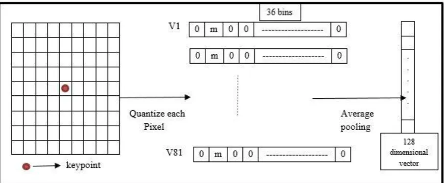
Extract low bit rate descriptors [23]. The number of descriptors depends on number of interest points. The following steps explain descriptors extraction, after drawing an m×n chunk around each interest point:
3.2.1 Smoothing step
Smooth chunk using two-dimensional Gaussian filter to remove noise using equation (1):
(1)
Where: σ is the standard deviation of the Gaussian distribution which determines the width of Gaussian filter. The
distribution is assumed to have a mean of 0. σ Is the variance of Gaussian filter.
3.2.2 Transformation step [23]
Map gradient vector and at every pixel calculate magnitude and orientation using equations (2 and 3):
(2)
(3)
Where: is image function.
is the derivative with respect to x (gradient in the x
direction).
is the derivative with respect to y (gradient in the y
measures change of intensity in the gradient direction.
is gradient direction.
3.2.3 Quantization step
Quantization step is used [23], one vector of length k will be obtained this vector is a zero vector except in one or two positions: at any pixel, if the gradient is (m, θ) and θi< θ < θi+1
i.e. θ lies between two quantization steps thus the corresponding vector of this pixel is: [0 0 0 0 0 0 0 mm 0 0 …0], however if θ has the same value of quantization step thus the corresponding vector of this pixel is: [0 0 0 0 0 0 0 0 0 m 0 0 …0]. Quantize orientation to k=36 directions to cover all orientation values. This step is equivalent to orientation binning in SIFT [8] descriptors which uses Also 36 bins histogram. Repeat step 3 for all pixels in the chunk, so matrix M of size k×b (k = m×n, b = binning number) will be obtained.
3.2.4 New patch vector average pooling step
Average pooling is applied to convert the matrix M from last step to give linear vector. Calculating average for each vector(row) in M independently such that each vector with length b will be represented by only one number after applying the average calculation for all rows (vectors in matrix M), one vector of length k will be obtained which describes interest point in this chunk. Unlike SIFT descriptor [8] in which the output of pooling stage are matrices by applying a square grid of pooling centers [23] using 8 bins histogram as Figure (1). Figure (2) declares the steps of constructing average proposed descriptor.
16x16 Window 128-dimensional vector
[image:3.595.82.262.400.510.2]
Keypoint
Fig. 1. SIFT a square grid pooling using 8 bins histogram
Repeat last steps for all chunks so Matrix MD (Matrix of Descriptors) of length (p×k), p= number of interest points will be obtained which contain all descriptors for input image.
Finally apply normalization by calculating the unit vector for each descriptor (each row in MD) to increase the robustness of descriptor by removing the dependence of descriptor on image contrast, using equation (4)
(4)
Where: is the unit vector is magnitude of the vector,
Compare input descriptors with the descriptors which are stored in database to get the perfect match. Suppose that input image descriptors matrix (MD), size(MD)=L and the descriptors matrices for each image in data base is MN where N is the data
base size And size
(M1)! = size (M2)! =…… size (MN)! Because each
image has specific number of descriptors and those numbers are not equal.
Calculate Euclidean distance [24] using equation (5) (5) Where: , are two vectors.
Finally select the image which has the min distance value.
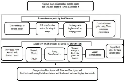
Figure (3) declares the steps of the proposed mobile visual search algorithm. Figure (3)
[image:3.595.73.527.536.723.2]Fig 3.A proposed mobile visual search algorithm
4.
RESULTS &DISCUSSION
4.1 Descriptors Extraction
This section discusses the running of the proposed method and monitor the obtained descriptors compared to the true descriptors existing in the tested image acquired via SIFT descriptor [8]. An image is captured via mobile, sent to server using web service (PHP-language), and processed. The database used consists of a number of 600 images: colored with various size jpg formats. It is deigned to be fast multi-scale “blob detector”, it works by computing an approximation of the image hessian’s determinant using (boxlets [25]) type features. Unlike traditional scale–space algorithms the feature is rescaled and is computed using integral image. Features are detected in a series of octaves; each octave is defined as a set of scales where higher octaves contain larger scales [14].
Before testing the algorithm, three parameters are introduced: = number of descriptors.
= time to measure the duration of descriptor matching between the query image and database images in SIFT [8].
= time to measure the duration of descriptor
matching the query image and database images in the proposed descriptor.
Table (1): shows validation for the proposed algorithm applied to five case studies under the same number of features (descriptors) in database. When the number of descriptors in the database increased from 353 to 5700 descriptors, the duration of descriptor matching time also increased as shown in Table 2.
Table (1): Descriptor matching time comparisonbetween Sift and proposed descriptor for small database Case
number
case І 72 2 sec 1 sec
Case п 93 2 sec 1 sec
case Ш 66 3 sec 1 sec
case IV 78 2 sec 1 sec
case V 44 2 sec 1 sec
Table (2): Descriptor matching time comparisonbetween Sift and proposed descriptor for large database Case
number
case І 72 14 sec 5 sec
Case п 93 15 sec 5 sec
case Ш 66 21 sec 4 sec
case IV 78 13 sec 4 sec
case V 44 15 sec 4 sec
So, it could be concluded that the Sift descriptor takes more time to match two sets of descriptors than the proposed descriptor, causing delay as time on big database increases as well.
4.2 Cropping Attack
[image:4.595.64.541.81.395.2]the number of IPs is reduced to k (k<K). However, when this nxn sub image is tested as an original one, the number of IPs is exceeding k as the algorithm begins searching for IPs relevant to this area. For this reason, two parameters are defined related to copping attack:
= number of descriptors that extracted in cropped area calculated from original image.
= number of descriptors that extracted in the cropped (when construed as a separate image).
= exact matched descriptors between original image and cropped image ratio.
(7)
(8) Usually , except if the cropped image does not contain special features. Furthermore, and could be equal but not similar descriptors. Table (3) displays case І: for high density fifteen descriptors in are found matched with their correspondents in and EMPC is sufficient for a true match. For low density two descriptors in are found matched with their correspondents in and EMPC is gives a
False match. From Table (3) it could be shown that the density of descriptors plays an important role in image matching. Table (4) displays results of other images for cropping part. From obtained results, it could be seen that the proposed algorithm achieves 100% EMPC.
Table (3): Cropping results for high and low-density interest points
case І original image High density patch Low density patch
=15 =2
=31 =24
EMPCS=100%
=20
EMPC=100%
Table (4): Cropping results for four different case studies Case
п
=18 =26 EMPC=100% true match Case
Ш
=13 =28 EMPC=100% true match Case
IV
=18 =22 EMPC=100% true match Case
V
=10 =21 EMPC=100% true match
4.3 Rotation Part
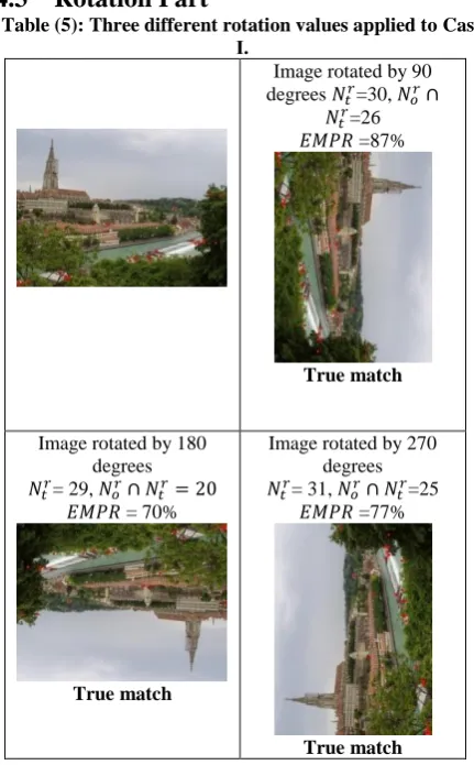
Table (5): Three different rotation values applied to Case І.
Case І Original image =30
Image rotated by 90 degrees =30,
=26 =87%
True match
Image rotated by 180 degrees = 29,
= 70%
True match
Image rotated by 270 degrees = 31, =25
=77%
True match
In rotation part similar parameters will be defined but named and .
: = , but the ‘r’ specifies rotation.
: Number of extracted descriptors after image rotation. =Exact matched descriptors between original image and rotated image ratio.
(9)
(10)
Rotation attack will be verified for images with different size. 50 images have been chosen randomly from database and tested at 90,180 and 270 degrees respectively. For 90 degrees, 11 images have been achieved wrong match. For 180 degrees, 9 images have been achieved wrong match. For 270 degrees, only one image from 50 has been achieved wrong match. The incoming results give adequate overview of how the algorithm performs.
[image:5.595.318.534.80.428.2] [image:5.595.47.291.406.532.2]achieves correct matching.
It could be concluded that; since the keypoint descriptor is represented relative to the orientation therefore it achieves invariance to image rotation.
Table (6): Results of four different cases for rotation part
Case degrees Matching
п 90 25 18 72% true match
180 25 18 72% true match
270 25 17 68% true match
Ш 90 23 17 73% true match
180 23 13 56% true match
270 23 17 73% true match
IV 90 28 25 89% true match
180 28 19 69% true match
270 28 22 78% true match
V 90 23 19 79% true match
180 23 17 74% true match
270 23 18 72% true match
4.4 Noise Attack
White Gaussian Noise (WGN) is applied on six cases to mimic the effect of many random processes that occur in nature. WGN is good approximation of other types of noise special when it is looked at small region of image or pixel values. In all selected images It should be taken in consideration the variation of the number of descriptors. : will be similar to , = .
: Number of extracted descriptors after adds noise to image.
=Exact matched descriptors between original image and noisy image ratio.
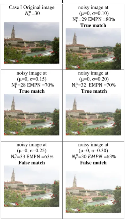
(11) (12) Applying WGN will be at constant mean (µ=0) and different variance values (σ=0.10, 0.15, 0.20, 0.25 and 0.30). Obtained results are show. Table (7) displays case І: for (µ=0, σ=0.10) twenty-four descriptors in are found matched with their correspondents in and are sufficient for a true match. For (µ=0, σ=0.15) twenty-one descriptors in are found matched with their correspondents in and is sufficient for a true match. For (µ=0, σ=0.20) twenty-one descriptors in are found matched with their correspondents in and is sufficient for a true match. However, for (µ=0, σ=0.25) nineteen descriptors in are found matched with their correspondents in and is sufficient for a false match. And for (µ=0, σ=0.30) nineteen descriptors in are found matched with their correspondents in and are sufficient for a false match.
Table (7): Noise Attack Results at different levels for Case І
Case І Original image =30
noisy image at (µ=0, σ=0.10) =29 =80%
True match
noisy image at (µ=0, σ=0.15) =28 =70%
True match
noisy image at (µ=0, σ=0.20) =32 =70%
True match
noisy image at (µ=0, σ=0.25) =33 =63%
False match
noisy image at (µ=0, σ=0.30) =30 =63%
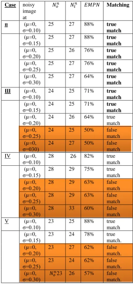
[image:6.595.320.537.86.466.2] [image:6.595.51.284.139.355.2]Table (8): Results of other cases for Noise Attack part
Case noisy
image at
Matching
п (µ=0, σ=0.10)
25 27 88% true
match (µ=0,
σ=0.15)
25 27 88% true
match (µ=0,
σ=0.20) 25 26 76% true match (µ=0,
σ=0.25) 25 27 76% true match (µ=0,
σ=0.30)
25 27 64% true
match Ш (µ=0,
σ=0.10)
24 25 71% true
match (µ=0,
σ=0.15)
24 25 71% true
match (µ=0,
σ=0.20) 24 26 64% true match (µ=0,
σ=0.25)
24 25 50% false
match (µ=0,
σ=030)
24 27 50% false
match IV (µ=0,
σ=0.10)
28 82% true
match (µ=0,
σ=0.15) 28 29 75% true match (µ=0,
σ=0.20) 28 29 63% false match (µ=0,
σ=0.25)
28 29 63% false
match (µ=0,
σ=0.30)
28 33 60% false
match V (µ=0,
σ=0.10)
23 25 88% true
match (µ=0,
σ=0.15) 23 24 78% true match. (µ=0,
σ=0.20) 23 27 62% false match. (µ=0,
σ=0.25) 23 24 62% false match. (µ=0,
σ=0.30)
23 26 57% false match.
4.5 Further study for processing time
By testing the proposed algorithm, it could be concluded that. There are two main factors effect correct matching and running time. The first factor is number of features since SURF detector is used by increasing number of features that return from non-maximum suppression algorithm [26], which responsible for select the most intensive features in scale space for each octave. The Second factor is the number of scales in each octave; increasing scales in octaves also increase features. So, by increasing features some cases that were achieved false match achieved a true match. But on the other side increase features causing increases in running time as a table (8) illustrates.
Table (8): displays some correct and incorrect matches in noise attack part after increase features from 20 to 100 features.
Assuming that:
is max number of features that return from non-maximum suppression algorithm.
: is time of matching process.
Table (9): Results for other cases after the increase in numbe r of feature s. (µ=0, σ=0.20) (µ=0, σ=0.25) (µ=0, σ=0.30) Case І =20 =100 =20 =100 =20 =100 false matc h true matc h se c false matc h 5 sec True matc h 20 sec Case Ш false matc h 4sec true matc h 21 sec false matc h 4 se true matc h 18 sec Case IV false matc h 4 sec true matc h 19 sec false matc h 4 sec true matc h se c false matc h 4 sec true matc h 18 sec Case V false matc h 4 sec false matc h 14 sec false matc h 5 sec false matc h 15 sec false matc h 6 sec false matc h 15 sec
Another parameter that had no significant effect is binning numbers, while increasing or decreasing orientation bins like (k=10, 19, and37) running time and matching didn’t change.
5.
CONCLUSION
[image:7.595.58.274.91.553.2] [image:7.595.311.548.115.497.2]performance the proposed system to rotation, illumination, scale, and noise.
6.
REFERENCES
[1] C. D Manning, P. Raghavan and H. Schütze. 2008. Introduction to information retrieval. Cambridge University Press.
[2] Mead Data Central. LEXIS. 1980. A Primer and LEXIS Quick Reference Manual. New York: Mead Data Central.
[3] . Girod, V. Chandrasekhar, D. M. Chen, N.M. Cheung, R. Grzeszczuk, Y. Reznik, G. Takacs, S. S. Tsai, R. Vedantha. 2011.Mobile visual search. IEEE signal processing magazine. vol. 28. no. 4. pp.61-76.
[4] B. Girod, V. Chandrasekhar, R. Grzeszczuk, Y. A. Reznik. 2011. Mobile visual search: Architectures, technologies, and the emerging MPEG standard. IEEE MultiMedia, vol. 18. no. 3. pp. 86-94.
[5] C. Schmid, R. Mohr, C. Bauckhage. 2000. Evaluation of interest point detectors. International Journal of computer vision. Vol. 37. issue 2. pp.151-172.
[6] Google Goggles, Available:
http://www.google.com/mobile/goggles/, last accessed date: July-2017.
[7] Y. Zheng, M. Z., Y. Song, H. Adam, U. Buddemeier, A. Bissacco, F. Brucher, T.-S. Chua, and H. Neven. 2009. Tour theworld: Building a web-scale landmark recognition engine. CVPR. IEEE. pp. 1085–1092. [8] D. Lowe. 2004. Distinctive image features from
scale-invariant keypoints. International Journal of Computer Vision. vol. 60. no. 2. pp. 91–110.
[9] G. Amato, F. Falchi, and P. Bolettieri. 2010. Recognizing Landmarks Using Automated Classification Techniques: an Evaluation of Various Visual Features. Advances in Multimedia (MMEDIA). pp. 78-83.
[10]D. S. Prasvita and Y. Herdiyeni. 2013. mobile application for medicinal plant identification based on leaf image. International Journal on Advanced Science, Engineering and Information Technology. Vol. 3. pp.103-104.
[11]S. S. Tsai, D. M. Chen, V. Chandrasekhar, G. Takacs, N.-M. Cheung,R.Vedantham, R. Grzeszczuk, and B. Girod. 2010. Mobile product recognition. ACM International Conference on Multimedia. Folrence. Italy. pp. 1587-1590.
[12]S. S. Tsai, D. M. Chen, G. Takacs, V. Chandrasekhar, R. Vedantham, R. Grzeszczuk, and B. Girod. 2010. Fast geometric re-ranking for image-based retrieval. International Conference on Image Processing. Hong Kong.
[13]D. M. Jang and Matthew Turk. 2010. Car-Rec: A real
time car recognition system. Proc. IEEE Workshop on Applications of computer vision. Kona. Usa. pp. 599-605.
[14]H. Bay, T. Tuytelaars, and L. Van Gool. 2006. SURF: Speeded Up Robust Features. Proc. Of European Conference on Computer Vision (ECCV). Graz. Austria. [15]Kooaba,Available:
https://www.crunchbase.com/product/kooaba-image-recognition-api#/entity, last accessed date: July-2017. [16]Opencv, Available: http://opencv.org, last accessed date:
July-2017.
[17]Lim, J. H., Chevallet, J. P., & Merah, S. N. 2004. SnapToTell: Ubiquitous information access from camera. Workshop on mobile and ubiquitous information access. [18]H. Kawaji, K. Hatada, T. Yamasaki, and K. Aizawa.
2010. Image-based indoor positioning system: fast image matching using omnidirectional panoramic images. Proc.ACM International Workshop on Multimodal pervasive video analysis. Florence. Italy. pp.1-4. [19]Y. Ke and R. Sukthankar. 2004. PCA-SIFT: a more
distinctive representation for local image descriptors. Proceedings of IEEE Conference on Computer Vision and Pattern Recognition. Vol. 1. pp. 511-517.
[20]M. Datar, N. Immorlica, P. Indyk, and V. S. Mirrokni. 2004. Locality-sensitive hashing scheme based on p-stable distributions. Proceedings of the 20th Annual Symosium on Computational Geometry. pp. 253-262. [21]S.S. Tasi,D. Chen, J.P.Siingh, and B. Girod. 2008.
Rate-efficient, real-time cd cover recognition on a camera-phone. Proceedings of ACM Intern. Conf. on Multimedia. Canada. pp.1023-1024.
[22]Boofcv, Available: http://boofcv.org, last accessed date: July-2017.
[23]M. Brown, G. Hua, and S. Winder. 2011. Discriminative learning of local image descriptors. IEEE transactions on pattern analysis and machine intelligence. vol.1. pp.43-57.
[24]P. Simard, Y. LeCun, JS. Denker. 1993. Efficient pattern recognition using a new transformation distance. Advances in neural information processing systems. pp. 50-58.
[25]P. Simard Eon, P. Y. Simard, P. Haffner, and Y. Lecun. 1999. Boxlets: a fast convolution algorithm for signal processing and neural networks. Advances in Neuralltiformation Processing Systems. MIT Press. pp. 571-577.