Economics Working Paper Series
2018/010
Inference in Nonparametric Series Estimation with
Specification Searches for the Number of
Series Terms
Byunghoon Kang
The Department of Economics
Lancaster University Management School
Lancaster LA1 4YX
UK
© Authors
All rights reserved. Short sections of text, not to exceed two paragraphs, may be quoted without explicit permission,
provided that full acknowledgement is given.
Inference in Nonparametric Series Estimation with Specification
Searches for the Number of Series Terms
Byunghoon Kang∗
Department of Economics, Lancaster University
First version December 9, 2014; Revised March 31, 2018
Abstract
Nonparametric series estimation often involves specification search over the different number
of series terms due to the unknown smoothness of underlying function. This paper considers
pointwise inference in the nonparametric series regression for the conditional mean and intro-duces test based on the supremum of t-statistics over different series terms. I show that proposed
test has correct asymptotic size and it can be used to construct confidence intervals that have
correct asymptotic coverage probability uniform in the number of series terms. With possibly
large bias in this setup, I also consider infimum of the t-statistics which is shown to reduce size distortions in such case. Asymptotic distribution of the test statistics, asymptotic size, and
local power results are derived. I investigate the performance of the proposed tests and CIs in
various simulation setups as well as an illustrative example, nonparametric estimation of wage
elasticity of the expected labor supply from Blomquist and Newey (2002). I also extend our inference methods to the partially linear model setup.
Keywords: Nonparametric series regression, Pointwise confidence interval, Smoothing
pa-rameter choice, Specification search, Undersmoothing.
JEL classification: C12, C14.
∗
1
Introduction
I consider the following nonparametric regression model;
yi =g0(xi) +εi,
E(εi|xi) = 0
(1.1)
where {yi, xi}ni=1 is i.i.d. with scalar response variable yi, vector of covariates xi ∈ Rdx, and
g0(x) =E(yi|xi =x) is the conditional mean function. Theory of estimation and inference is well developed for nonparametric series (sieves) methods in large econometrics and statistics literature,1
and series estimation has also received attention in applied economics as it can easily impose
shape restrictions such as additive separability or monotonicity. However, implementation requires a choice of smoothing parameter, the number of series terms K = Kn, and this often involves specification searches, i.e., search over different series terms K∈ Kn= [K,K¯]. Existing theory for the asymptotic normality and valid inference imposes so-called undersmoothing (i.e., overfitting) condition that is a faster rate of K than the mean-squared error (MSE) optimal convergence rates, however, to achieve undersmoothing one has to know the smoothness of g0(x) which is
usually unknown in practice. Specification searches seem necessary in such case, but it may lead to misleading inference without taking into account the first step specification search.
This paper provides inference methods in nonparametric series regression given the range of the
different number of series terms. I consider the testing problem for a regression function at a point, and I show that (1) test based on the absolute value of supremum of the studentized t-statistics over
different series terms and its asymptotic critical value control the asymptotic size; (2) this test can be used to construct asymptotically valid confidence intervals (CI) which are uniform inK ∈ Kn; (3) in consequence, CI with any Kb ∈ Kn has a correct asymptotic coverage for g0(x) by adjusting
the conventional normal critical value to the critical value from supremum of the t-statistics. The main contribution of this paper is to derive a uniform asymptotic distribution theory
for the entire sequences of t-statistics over a range of the number of series terms K. Existing asymptotic normality of the t-statistic in the literature holds under a deterministic sequence of
K → ∞ asn→ ∞. First, I develop an asymptotic distribution of t-statistics over the set Kn that includes a finite number of sequences allowing a broad range of K from oversmoothing rates to undersmoothing rates as well as optimal MSE rates. In addition, I provide an empirical process theory for the t-statistics indexed by continuous parameterπ, a fraction of the largest series terms
¯
K, by considering different Kn; although this set assumption only allow same rates of K (put it differently,Kn can be small), it is sufficient to show the weak convergence of the empirical process. I also show that, in the special case, limiting Gaussian process coincides with the scaled Brownian
motion process so that the asymptotic critical value of the test statistics can be tabulated easily as
it is only a function of π =K/K¯ with the smallest K and the largest ¯K, and this can be viewed
1For examples, Andrews (1991a), Newey (1997), Huang (2003a), Chen (2007), Belloni, Chernozhukov, Chetverikov,
as an analogous result developed in the kernel estimation literature (for example, Armstrong and
Koles´ar (2015)).
With an asymptotic distribution theory established in the paper, I also consider tests based
on infimum of the t-statistics, and searching for “small” t-statistics in this setup has a similar
motivation with the undersmoothing assumption; using “large” K (or faster rates of K than the optimal MSE rate) which has a small bias and large variance, thus lead to “small” t-statistics.
For valid inference, many papers in nonparametric series estimation literature typically suggested
to increase the number of series terms and include additional terms than that cross-validation chooses (for example, see Newey, Powell, and Vella (1999), Newey (2013)), mainly due to the lack
of an explicit asymptotic bias formula and bias-corrections for the series estimator. I formally
justify this conventional wisdom by introducing the infimum test statistic overKn and provide an inference method based on its asymptotic distribution. We can, in principle, consider other “small”
t-statistics (e.g., 2nd smallest or median), but a valid pointwise CI can be constructed easily by
inverting infimum t-statistics; it is obtained as the union of all CIs by replacing the standard normal critical value with the critical value from the infimum t-statistic.
This paper also establishes asymptotic local power results for a particular sequence of slower
than n−1/2-local alternatives and show the size-power trade-off between supremum and infimum test statistics; similar to using undersmoothing rates, the test based on the infimum t-statistics
can reduce size distortion, but may also reduce the power of the tests. Formally, I show that the test based on the supremum test statistics is consistent against some sequences of local alternatives
while infimum test statistic is consistent only against a limited range of local alternatives. However,
the test based on infimum t-statistics controls the asymptotic size even allowing large asymptotic bias, and it has nontrivial power against some local alternatives, and has better power than the test
based on single t-statistic using normal critical value with “large”K that is faster than or equal to the optimal MSE rates.
I also provide a construction of valid CIs by test statistic inversion and show coverage results
of the proposed CIs. The critical values can be easily implemented using the asymptotic Gaussian
distribution. I investigate finite sample coverage and length properties of the proposed CIs in various simulation setups. As an illustrative example, I revisit nonparametric estimation of labor supply
function using entire individual piecewise-linear budget set as in Blomquist and Newey (2002).
Imposing additive separability, derived by economic theory, Blomquist and Newey (2002) estimate conditional mean of labor supply function using series estimation and report wage elasticity of the
expected labor supply as well as other welfare measures with various specifications of the different
number of series terms.
Finally, I provide inference methods in partially linear model setup focusing on the common
parametric part. Unlike the nonparametric object of interest that has a slower convergence rate
than n1/2 (e.g., regression function or regression derivative), t-statistics for the parametric object of interest are asymptotically equivalent for all sequences of K under standard rate conditions
Ks in this setup, I develop an asymptotic distribution of the studentized t-statistics over K ∈ Kn using the results of Cattaneo, Jansson, and Newey (2015a) under the faster rate of K that grows as fast as the sample size n. I also discuss methods to construct CIs that are similar to the nonparametric regression setup and provide coverage properties.
The supremum t-statistics has been used as a correction for the multiple testing problems or to construct simultaneous confidence bands, and the importance of multiple testing problems (data
mining or data snooping) has long been alerted in various other contexts (see Leamer (1983),
White (2000), Romano and Wolf (2005), Hansen (2005)). While considering infimum t-statistics is closely related to the undersmoothing assumption that conceptually requires increasingK until t-statistic is “small enough” in our nonparametric setup, it is also related to the “stepup” procedures
in the multiple testing literature (see, for example, Romano and Shaikh (2006)) which start by considering smallest test statistics (the least significant hypotheses) and then move up to the larger
test statistics. Furthermore, inference methods using the union of confidence intervals also has
been used in various contexts, for examples, instrumental variable (IV) setup without imposing instrument exclusion restriction as in Conley, Hansen, and Rossi (2012), sensitivity analysis in
parametric setup as in Levine and Renelt (1992) following Leamer (1983). With the bias-variance
trade-off of nonparametric estimators in our different setup, we provide less conservative inference methods from our asymptotic distribution results of the infimum test statistic with the critical
values smaller than the standard normal critical values.
Several important papers have investigated the asymptotic properties of series (and sieves)
estimators, including papers by Andrews (1991a), Eastwood and Gallant (1991), Newey (1997),
Chen and Shen (1998), Huang (2003a), Chen (2007), Chen and Liao (2014), Chen, Liao, and Sun (2014), Belloni et al. (2015), and Chen and Christensen (2015b), among many others. This paper
extends the asymptotic normality of the t-statistic under a single sequence of K to the uniform central limit theorem of the t-statistic for the sequences of K over a set Kn, and focuses on a pointwise inference ong0(x) which is an irregular (i.e., slower than n1/2 rate) and linear functional
under i.i.d. setup.
There is also a growing literature on data-dependent series term selection and its impact on estimation and inference in econometrics and statistics. Asymptotic optimality results of
cross-validation have been developed, including papers by Li (1987), Andrews (1991b), Hansen (2015).
Recent papers by Horowitz (2014), Chen and Christensen (2015a) develop data-driven methods for choosing sieve dimension in the nonparametric instrumental variables (NPIV) estimation so
that resulting NPIV estimators attain the optimal sup-norm or L2 norm rates adaptive to the unknown smoothness ofg0(x). Although we do not pursue adaptive inference in this paper, there
is also a large statistics literature on adaptive inference (see Gin´e and Nickl (2015, Section 8) for
comprehensive lists of references). For example, Gin´e and Nickl (2010), Chernozhukov, Chetverikov,
and Kato (2014a) construct adaptive confidence bands in density estimation problem. For regression setup, similar techniques developed in Chernozhukov et al. (2014a) can be used to approximate
asymptotic distributions in this paper can be useful to consider other test statistics, such as infimum
t-statistic, in pointwise inference. Furthermore, once data-driven choice is obtained for adaptive estimation (e.g., Lepski (1990)-type procedures), one still require undersmoothing condition for
inference to eliminate asymptotic bias terms (see Theorem 1 of Gin´e and Nickl (2010), and Corollary
3.1 of Chernozhukov et al. (2014a)), and this may come up with similar specification search issues to choose sufficiently “large”K in practice.
We can, in principle, consider kernel-based estimation where several data-dependent bandwidth
selections or explicit bias-corrections have been proposed,2 however, there exist many examples estimating g0(x) using series estimation with imposing shape constraints easily (such as additive
separability) and also interested in pointwise inference (see Section 7 for the example as in Blomquist
and Newey (2002)). Unlike the kernel-based methods, little is known about the statistical properties of data-dependent selection rules or an asymptotic theory for the bias-correction due to the lack of
an explicit asymptotic bias formula for the series estimator.3 With the issues of specification search,
this paper is closely related to a recent paper by Armstrong and Koles´ar (2015) which considers similar inference methods forg0(x) using kernel estimation with bandwidth snooping. We provide
coverage results that are uniform in series terms, as well as analogous limiting distributions for the
supremum of Gaussian processes as in Armstrong and Koles´ar (2015).
The rest of the paper is organized as follows. I introduce basic nonparametric series regression
setup and the asymptotic distribution in Section 2 and the asymptotic size and power properties of the test statistics in Section 3. In Section 4, I introduce CIs, implementation of the critical values
and provide coverage results. Section 5 extends our inference methods to the partially linear model
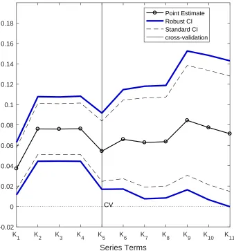
setup. Section 6 summarizes Monte Carlo experiments in various setups, and Section 7 illustrates empirical example as in Blomquist and Newey (2002), then Section 8 concludes. Appendix A
includes all proofs, and Appendix B includes figures and tables.
1.1 Notation
I introduce some notation will be used in the following sections. I use ||A|| = ptr(A0A) for the Euclidean norm. Let λmin(A), λmax(A) denote the minimum and maximum eigenvalues of a symmetric matrix A, respectively. op(·) and Op(·) denote the usual stochastic order symbols, convergence in probability and bounded in probability. −→d denotes convergence in distribution and ⇒ denotes weak convergence. I use the notation a∧b = min{a, b}, a∨b = max{a, b}, and denote bac as the largest integer less than the real number a. For two sequences of positive real numbersan and bn, an.bn denotesan≤cbn for all nsufficiently large with some constant c >0 that is independent of n. anbn denotesan.bn andbn.an. For a given random variable{Xi} and 1≤p <∞,Lp(X) is the space of allLpnorm bounded functions with||f||Lp= [E||f(Xi)||p]1/p
and `∞(X) denotes the space of all bounded functions under sup-norm,||f||∞= supx∈X|f(x)|for
2
See H¨ardle and Linton (1994), Li and Racine (2007) for references. See also Hall and Horowitz (2013), Calonico, Cattaneo and Farrell (2015), Schennach (2015) and references therein for various recent works on related bias issues and inference for the kernel estimator.
3
the bounded real-valued functions f on the support X. Let alsoR[±∞]=R∪ {+∞} ∪ {−∞}.
2
Model framework and asymptotic distribution
I first introduce the nonparametric series regression setup in the model (1.1). Given a random
sample {yi, xi}ni=1, we are interested in the conditional mean g0(x) = E(yi|xi = x) at a point
x∈ X ⊂Rdx. All the results derived in this paper are the pointwise inference in x, and I will omit
the dependence on xif there is no confusion.
Let bgn(K, x) be an estimator of g0(x) using the first K = Kn ≥ 1 series terms PK(x) = (p1(x),· · ·, pK(x))0 from basis functionsp(x) = (p1(x), p2(x),· · ·)0. Standard examples for the basis
functions are power series, Fourier series, orthogonal polynomials (e.g., Hermite polynomials), or
splines with evenly sequentially spaced knots. Series estimator is then obtained by standard least square (LS) estimation of yi on regressors PK(xi)
b
gn(K, x) =PK(x)0βbK, βbK= (PK
0
PK)−1PK0Y (2.1)
where PK = [PK1,· · ·, PKn]0, PKi ≡ PK(xi) = (p1(xi), p2(xi),· · ·, pK(xi))0, Y = (y1,· · ·yn)0. For simplicity of notation, I define the true regression function at a point asθ0≡g0(x) and letθbn(K)≡ b
gn(K, x). Define the series variance
Vn(K)≡Vn(K, x) =PK(x)0Q−K1ΩKQ−K1PK(x),
QK =E(PKiPKi0 ), ΩK =E(PKiPKi0 ε2i)
(2.2)
whereQ−K1ΩKQ−K1 is the conventional asymptotic variance formula for the LS estimatorβbK.
We use the notion of testing setup and consider two-sided testing for θ
H0 :θ=θ0, H1 :θ6=θ0. (2.3)
The studentized t-statistic forH0 is
Tn(K, θ0)≡
√
n(bgn(K, x)−g0(x))
Vn(K, x)1/2
= √
n(θbn(K)−θ0)
Vn(K)1/2
. (2.4)
Under standard regularity conditions (will be discussed below in Assumption 2.2), t-statistic under
H0 can be decomposed as follows
Tn(K, θ0) =
1 √
n
n
X
i=1
PK(x)0Q−K1PKiεi
Vn(K)1/2
− prn(K)
Vn(K)/n
+op(1) (2.5)
(E[PKiPKi0 ])−1E[PKiyi]. With undersmoothing assumption, the asymptotic distribution of the t-statistic,Tn(K, θ0)−→d N(0,1), is well known in the literature (See, for example, Andrews (1991a),
Newey (1997), Belloni et al. (2015), Chen and Christensen (2015b) among many others), and the
confidence interval for the nonparametric regression function can be constructed.
Here, I develop an asymptotic distribution theory ofTn(K, θ0) over a setKn. The following set assumption is constructed to allow a broad range of Ks so thatKn can allow (unknown) optimal mean squared error rate ofK as well as oversmoothing rate which increases slower than the optimal MSE rate.
Assumption 2.1. (Set of number of series terms) Let Kn as
Kn = {K = K1,· · ·, Km,· · ·,K¯ = KM} where Km ≡ bτ nφmc for constant τ > 0, 0 <
φ1 < φ2 < · · · < φM, and fixed M. Define asymptotic bias for the m-th model as ν(m) ≡
− lim n→∞
√
nVn(Km)−1/2rn(Km). Assume that infm|ν(m)|=O(1).
Remark 2.1. Suppose g0(x) belongs to the H¨older space of smoothness s >0, Σ(s,X), then we
obtain optimal L2 convergence rates Op(n−s/(2s+dx)) with K ndx/(dx+2s). Due to the unknown smoothness of g0(x), Kn may include small Ks corresponding to oversmoothing rates. If the unknown optimal MSE rates satisfy φp < dx/(dx+ 2s)≤φp+1 for some p∈ {1,· · ·, M −1}, then
Assumption 2.1 contains oversmoothing rates ofK (|ν(m)|= +∞ for all m= 1,· · ·, p), as well as optimal MSE rate and undersmoothing rates (|ν(p+1)|<+∞,|ν(m)|= 0 for allm=p+2,· · ·, M). Also note that infm|ν(m)|=O(1) excludes the possibility of |ν(m)|= +∞ for all m= 1,· · ·, M.4 We may consider growing set of the possible number of series terms withKn= [K,K¯]∩N(similar
assumption is used in the literature, for example, Newey (1994a, 1994b)), but this complicates the
derivation of the limiting distribution. We can use the general results of Chernozhukov, Chetverikov, and Kato (2013) in this case, however, obtaining asymptotic distributions over K ∈ Kn is useful in our pointwise inference setup to consider other test statistics. We also consider different Kn
including infinite sequences ofK in Section 2.1 to establish weak convergence results.
Next, I impose mild regularity conditions that are standard in nonparametric series
regres-sion literature and are satisfied by well-known basis functions. For each K ∈ Kn, define ζK ≡ supx∈X||PK(x)||as the largest normalized length of the regressor vector andλK ≡(λmin(QK))−1/2 forK×K design matrixQK =E(PKiPKi0 ).
Assumption 2.2. (Regularity conditions)
(i) {yi, xi}ni=1 are i.i.d random variables satisfying the model (1.1).
4Assumption 2.1 allows to have optimal L2 rates of K in a large set of classes of functions; by setting φ
m =
(ii) supx∈XE(ε2i|xi =x)<∞, infx∈XE(ε2i|xi =x)>0, andsupx∈XE(ε2i{|εi|> c(n)}|xi =x)→
0 for any sequence c(n)→ ∞ as n→ ∞.
(iii) For each K ∈ Kn, as K → ∞, there existsη and cK, `K such that
sup x∈X
|g0(x)−PK(x)0η| ≤`KcK, E[(g0(xi)−PK(xi)0η)2]1/2 ≤cK.
(iv) supK∈KnλK .1.
(v) supK∈KnζK
p
(logK)/n(1 +√K`KcK) +`KcK →0 as n→ ∞.
Assumption 2.2(ii) imposes moment conditions and standard uniform integrability conditions.
Assumption 2.2(iii)-(v) are similar to those imposed in Belloni et al. (2015), Chen and Christensen
(2015b) except that we impose rate conditions ofK uniformly overKn. Other standard regularity conditions in the literature (e.g., Newey (1997), Chen (2007)) can also be used here, soζK, cK, `K in Assumption 2.2(iii)-(v) are satisfied with various sieve bases and all the discussions made there
also apply here.5
Next theorem provides an asymptotic distribution under Assumption 2.1 with a broad range
of K. Allowing supm|ν(m)| = +∞ in the result will be useful for considering the effect of bias on the asymptotic size of the test, as well as for obtaining asymptotic distributions of the test statistics under the wide range of local alternatives. For this, we define the continuous function on
the extended real space as follows; S :A → B is continuous at t ∈ A if t0 → t for t ∈A implies
S(t0)→S(t) for any setA.
Theorem 2.1. Under Assumptions 2.1 and 2.2, following holds for any continuous functionS(t)
at all t∈ T ⊂RM
[±∞],
S(Tn(θ0)) d
−→S(ZΣ+ν)
where Tn(θ) = (Tn(K1, θ),· · ·, Tn(KM, θ))0, ZΣ = (Z1,· · ·, ZM)0 ∼ N(0,Σ), ν = (ν(1),· · ·, ν(M))0
are M ×1 vectors provided that Σ exists and is a finite positive definite matrix with Σ(j, l) =
limn→∞Σn(j, l), and
Σn(j, l) =
PKj(x) 0E(P
KjiP 0
Kji) −1E(P
KjiP 0
Kliε
2
i)E(PKliP 0
Kli) −1P
Kl(x)
Vn(Kj)1/2Vn(Kl)1/2
.
5For example, if the supportX is a cartesian product of compact connected intervals (e.g. X = [0,1]dx) and the
probability density ofxiis bounded below zero, thenζK .Kfor power series and other orthogonal polynomial series, andζK .
√
If ν(m) =±∞, then the corresponding element of ZΣ+ν equals ±∞.
This is an asymptotic theory for the entire sequence of t-statistics Tn(K, θ0), K ∈ Kn. Note that standard inference methods in nonparametric regression setup typically consider a singleton set Kn={K}withK → ∞ asn→ ∞.
Remark 2.2. We note that Theorem 2.1 does not require either undersmoothing assumption for all K ∈ Kn or supm|ν(m)|<∞. The t-statistics may not converge in distribution to a bounded random vector if|ν(m)|= +∞for somem; corresponding t-statisticTn(Km, θ0) diverges in
proba-bility to±∞. This matters when we obtain the asymptotic distribution of the test statistic because continuous mapping theorem cannot be directly applied. To obtain the asymptotic distribution
un-der supm|ν(m)|= +∞, we provide formal proofs which combine arguments in inference on CIs for the parameters in moment inequality literature as in Andrews and Guggenberger (2009).6 Theorem 2.1 coincides with standard continuous mapping theorem when we control maximum asymptotic
bias or impose uniform undersmoothing assumption (i.e., supm|ν(m)| = 0), and thus useful to analyze the effect of large bias on the size of the tests, and to compare the power of asymptotic
levelα tests under wide range of local alternatives (see Section 3.1 and 3.2 for details).
Remark 2.3 (Variance-covariance matrix). Under conditional homoskedasticity, E(ε2i|xi =x) =
σ2, variance-covariance matrix Σ reduces to the simple form as Σ(j, l) = limn→∞Vn(Kj∧Kl)
1/2
Vn(Kj∨Kl)1/2,
i.e., the limit of the ratio of standard deviations. If we assume Vn(K)1/2 Kη at some point x with η > 0, then for any j < l, Σn(j, l) ≤ CVn(Kj)
1/2
Vn(Kl)1/2 for some constant C > 0 by Assumption
2.2(ii) and the upper bound converges to 0 as n → 0 by Assumption 2.1, thus Σn(j, l) → 0 and variance-covariance matrix also reduces to Σ =IM.
Remark 2.4(Other functionals). Here, we focus on the leading example, whereθ0 =g0(x) for some
fixed pointx∈ X, but we can consider other linear functionalsθ0=a(g0(·)), such as the regression
derivates a(g0(x)) = dxdg0(x). All the results in this paper can be applied to irregular (slower than
n1/2 rate) linear functionals using estimators bθn(K) = a(gbn(K, x)) = aK(x)0βbK and appropriate
transformation of basis aK(x) = (a(p1(x),· · ·, a(pK(x)))0 with proper smoothness condition on the functional and continuity conditions on the derivative as in Newey (1997). While verification of
previous results for regular (n1/2rate) functionals, such as integrals and weighted average derivative, is beyond the scope of this paper, I examine similar results for the partially linear model setup in
Section 5.
Remark 2.5(LargestK). Although there exist rate restrictions for ¯Kto be used for the asymptotic normal approximation, formal guidance or data-dependent results for the range ofKn= [K,K¯] are beyond the scope of this paper. Together with Assumption 2.2, there exist explicit rate restrictions
on φm in the Assumption 2.1 uniformly over m to guarantee asymptotic normality of single t-statistic. For example, under supK∈KnK
2logK/n→0 for the power series, rates are allowed only
6
ifφM <1/2. Some formal data-dependent methods to obtain optimalL2 norm or sup-norm rates, such as cross-validation can be useful guidelines for Kn, and it would be of interest to extend all inference results developed in this paper with data-dependentKn.
2.1 Weak convergence of t-statistic process
In this section, I consider different set assumptionKnto construct empirical process theory of the
t-statistics overK ∈ Knwhich I shall call ‘t-statistic process’. The t-statistic process is indexed by the continuous and fixed parameter π, which is a fraction of the largest series term ¯K.
Assumption 2.3. (Same Rates of K) Let Kn as
Kn={K :K ∈[πK,¯ K¯]}
where K = πK¯ with a fixed constant π ∈ Π = [π,π¯], 0 < π < π¯ = 1, and K¯ ≡ K¯(n) → ∞ as
n→ ∞.
Assumption 2.3 considers a range of the number of series terms and considers an infinite sequence of approximations indexed by π ∈ Π. By imposing the rate conditions for the largest series term
¯
K with the Assumption 2.2, set Knconsiders the sequence of models that has the same rate ofK, i.e., K K0 for anyK, K0 ∈ Kn.
Next, define the following empirical process, Tn∗(π, θ), as
Tn∗(π, θ)≡Tn(bπK¯c, θ), π∈Π, (2.6)
where Tn(K, θ) is defined in (2.4), i.e.,Tn∗(π, θ) is a t-statistic evaluated at the parameter θ using
bπK¯c number of series terms. Note that Tn∗(π, θ) is indexed by π∈Π and is a step function of π. This empirical process has a covariance kernel
Σn(π1, π2)≡
Pπ1(x)
0Q−1
π1E(Pπ1iP
0
π2iε
2
i)Q−π21Pπ2(x)
Vn(π1)1/2Vn(π2)1/2
, π1, π2 ∈Π, (2.7)
where Pπ(x) ≡ PbKπ¯ c(x), Pπi ≡ Pπ(xi) = PbKπ¯ ci, and the series variance Vn(π) ≡ Vn(bπK¯c,
x) =||Ω1π/2Qπ−1Pπ(x)||2, Ωπ =E(PπiPπi0 ε2i), Qπ =E(PπiPπi0 ). We expect that the limiting Gaussian process has a covariance function as a limit of the sequence of covariance functions Σn(π1, π2), which
is assumed to exist by the following assumption. To establish weak convergence of the empirical
process{Tn∗(π, θ0) :π ∈Π}, I also impose rate restrictions on series variances.
Assumption 2.4.
(i) Σ(π1, π2) = limn→∞Σn(π1, π2) exists andΣ(π1, π2)<1 for anyπ1, π2 ∈Π.
Assumption 2.4(i) guarantees well-defined covariance function for the tight Gaussian process in
`∞(Π) and a positive definite variance-covariance matrix for its finite-dimensional limit distribu-tions. Assumption 2.4(ii) is a high-level assumption but required to prove weak convergence of the
t-statistic process. Assumption 2.4(ii) requires that series variance is increasing inK at some rates uniformly inK ∈ Knunder Assumption 2.3, i.e., limn→∞Vn(K)1/2K−η =c. This assumption holds with η = 1/2 when we consider a point x ∈ X where Vn(K)1/2 ∝ K1/2. Moreover, Assumption 2.4(ii) is a sufficient condition for Assumption 2.4(i) under homoskedasticity. Under conditional
homoskedasticity, E(ε2i|xi=x) =σ2, the limit of the covariance kernel Σ(π1, π2) reduces to the
Σ(π1, π2) = lim n→∞
Vn(π1∧π2)1/2
Vn(π1∨π2)1/2
(2.8)
for any π1, π2 ∈ Π. If we further assume Assumption 2.4(ii), then Σ(π1, π2) = (ππ11∧∨ππ22)
η. With
η = 1/2, this coincides with the covariance kernel of a scaled Brownian motion process Z(π)/
√
π, π∈Π.
Next, we define the asymptotic bias as ν(π) ≡ limn→∞−
√
nVn(π)−1/2rn(π) for π ∈ Π, where
rn(π) ≡rn(bπK¯c, x) and consider undersmoothing assumption. Under Assumption 2.5,ν(π) = 0 for all π∈Π.7
Assumption 2.5. (Undersmoothing) sup K∈Kn
|√nVn(K)−1/2rn(K)| →0 as n→ ∞.
Next theorem provides uniform central limit theorem of the t-statistic process for nonparametric LS series estimation.
Theorem 2.2. Under Assumptions 2.2, 2.3, 2.4 and supπ|ν(π)|<∞,
Tn∗(π, θ0)⇒T(π) +ν(π), π∈Π, (2.9)
where T(π) is a mean zero Gaussian process on `∞(Π) with covariance kernel, E(T(π1)T(π2)) =
Σ(π1, π2) for anyπ1, π2 ∈Π, defined in Assumption 2.4. In addition, if Assumption 2.5 is satisfied,
then
Tn∗(π, θ0)⇒T(π), π∈Π. (2.10)
Theorem 2.2 provides weak convergence of the t-statistic process Tn∗(π, θ0), π ∈ Π. The
t-statistic process converges weakly to a mean zero Gaussian processT(π) plus the asymptotic bias
ν(π). Proof of Theorem 2.2 needs to verify a uniform-entropy condition and apply empirical process theory in van der Vaart and Wellner (1996, Theorem 2.11.22).
7
When we use explicit bounds`KcK .K−s/dx for spline or wavelet series, sufficient condition for Assumption 2.5 is sup
K∈Kn
√
Remark 2.6 (Rate conditions). Theorem 2.2 requires supπ|ν(π)| < ∞ so that t-statistics has either zero asymptotic bias for all K ∈ Kn or non-zero bounded asymptotic bias for all K ∈ Kn. A setKnin Assumption 2.3 allows narrower ranges ofK than the Assumption 2.1 because it only considers sequences of K with the same rates which only differ in constant π. However, these are the class of sequences to be able to provide uniform central limit theorem of the t-statistic process; as discussed in Remark 2.3, studentized t-statistic can be asymptotically independent with
different rates of K. Moreover, weak convergence results can be used for tabulating critical value (see Remark 4.1 for more details).
3
Test statistic
In this section, I introduce test statistics and analyze its asymptotic null distribution based on Theorem 2.1. Then, I provide an asymptotic size result of the tests and consider local power
analysis (I restrict attention to Assumption 2.1 which considers a more general range of Kn than
Assumption 2.3, and thus power results under Theorem 2.2 are omitted for brevity). I consider following supremum and infimum test statistics,
SupTn(θ) = sup K∈Kn
|Tn(K, θ)|,
InfTn(θ)≡ inf K∈Kn
|Tn(K, θ)|.
(3.1)
As I denoted in the introduction, considering SupTn(θ) is appropriate in the context of multiple testing and is known to control the size of the simultaneous tests over Kn. There are also several
reasons to consider InfTn(θ) in the series regression context; small t-statistic centered at the true
θ0 corresponds to the approximation that has a small bias and large variance, similar to
under-smoothing assumption. Using similar ideas of some rule-of-thumb methods suggested to choose
undersmoothed series terms, I provide formal inference methods based on asymptotic distribution results of the infimum test statistic with appropriate critical values smaller than the standard
normal critical values.8 Using infimum t-statistics is also related to certain sensitivity analysis in
the parametric setup, such as Levine and Renelt (1992) following Leamer (1983)’s idea, which is so-called Leamer’s “Extreme Bounds Analysis.”9
Asymptotic null limiting distribution of the test statistic follows immediately from Theorem
2.1.
8
For example, among many others, Newey (2013) suggested increasingKuntil standard errors are large relative to small changes in objects of interest, Newey, Powell, and Vella (1999) suggested using more terms than that cross-validation chooses, and Horowitz and Lee (2012) suggested increasingKuntil the integrated variance suddenly increases and then adding an additional term.
9
In the parametric setup, a variable is defined as “robust” when 0 is not included in the lower and upper extremes ofθbn(m)±1.96s(θbn(m)) over different specificationsm= 1,· · ·, M, otherwise “fragile”. This is easily shown to be equivalent to testing InfTn(0) = infm|
b
θn(m)
Corollary 3.1. Under Assumptions 2.1, 2.2 and,supm|ν(m)|<∞ , then
SupTn(θ0) d
−→ξsup(Σ, ν)≡ sup m=1,···,M
|Zm+ν(m)|, (3.2)
whereZm is an element ofM×1 normal vectorZΣ∼N(0,Σ) andν = (ν(1),· · ·, ν(M))0 is defined
in Theorem 2.1. Under Assumptions 2.1, 2.2,
InfTn(θ0)−→d ξinf(Σ, ν)≡ inf
m=1,···,M|Zm+ν(m)|. (3.3)
Corollary 3.1 gives the asymptotic distribution of our test statistics, SupTn(θ) and InfTn(θ). In addition, if Assumption 2.5 holds, then the limiting distributions ξsup(Σ,0M) and ξinf(Σ,0M) do not contain bias components. Allowing supm|ν(m)|= +∞for some m, InfTn(θ0) converges in
distribution to the bounded random variable, while SupTn(θ0) converges in probability to infinity.
Using InfTn(θ) can reduce size distortions, however, it may have low power; similar to the size and power trade-off using (deterministic) undersmoothing rates compare with slower than or equal to
the optimal MSE rates. We investigate this trade-off between size and power of the test in the
following sections.
3.1 Asymptotic size
I start by defining critical valuecsup1−α(ν), cinf1−α(ν) for 0< α <1/2,
csup1−α(ν) =Fξ−1
sup(Σ,ν)(1−α), c
inf
1−α(ν) =Fξ−inf1(Σ,ν)(1−α) (3.4)
where FX−1(1−α) denotes the (1−α) quantile of the random variableX. I also define z1−α/2 as
(1−α/2) quantile of the standard normal random variable, which solves P(|Z| > z1−α/2) = α,
Z ∼N(0,1).
Next Corollary provides the asymptotic size of the test based on SupTn(θ) with the critical valuecsup1−α(ν).
Corollary 3.2. Under Assumptions 2.1, 2.2, andsupm|ν(m)|<∞, following holds
lim
n→∞P(SupTn(θ0)> c sup
1−α(ν)) =α. (3.5)
Moreover,
lim sup n→∞
P(Tn(K, θb 0)> c
sup
1−α(ν))≤α (3.6)
for anyKb ∈ Kn.
value from supremum test statistics will also be valid, but conservative.
Next Corollary provides the asymptotic size of the tests based on InfTn(θ).
Corollary 3.3. Under Assumptions 2.1 and 2.2, following holds,
lim
n→∞P(InfTn(θ0)> c inf
1−α(ν)) =α. (3.7)
Corollary 3.3 shows that the tests based on InfTn(θ) asymptotically control size without as-suming supm|ν(m)|<∞. Even when we allow “large” asymptotic bias (|ν(m)|=∞) for several
Ks inKn, size of the test is asymptotically level α.
Remark 3.1. Note that InfTn(θ0) ≤ |Tn(Km, θ0)| and |Tn(Km, θ0)| d
→ |N(ν(m),1)| for any single Km ∈ Kn, thus we can also show that the test based on InfTn(θ) using critical value infmF|−N1(ν(m),1)|(1−α) controls the asymptotic size, but conservative. Note that infmF|−N1(ν(m),1)(1−
α)|=F|−N1(ν( ˆm),1)(1−α) with ˆmsuch that|ν( ˆm)|= infm|ν(m)|and this coincides with normal crit-ical valuez1−α/2when infm|ν(m)|= 0, which implies that the test based on InfTn(θ0) with normal
critical value controls size asymptotically if the smallest asymptotic bias is 0, which is the case when Kn includes at least one undersmoothing sequence.
3.2 Asymptotic local power properties
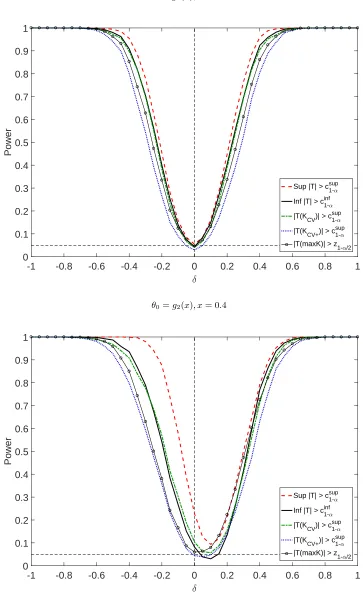
In this section, we investigate the local asymptotic power of the tests based on SupTn(θ) and InfTn(θ).10
In order to establish the power properties of our test, we impose following assumptions.
Assumption 3.1.
(i) Let θn=θ0+ ¯µn−γ for some µ¯∈R and γ >0.
(ii) pn/Vn(Km) nδm for all Km ∈ Kn defined in Assumption 2.1 such that 1/2 > δ1 > δ2 >
· · ·> δM >0.
The local alternatives are defined in 3.1(i) and high-level assumption 3.1(ii) is used to charac-terize the asymptotic distribution under local alternatives. Since nonparametric estimator θbn(K)
is converging at a rate pn/Vn(K), we need rate restrictions on series variance Vn(K) similar to Assumption 2.4(ii) to compare rates ofpn/Vn(K) and n−γ, as well as asymptotic bias term.
Under Assumptions 2.1, 2.2 and 3.1, limiting distribution of the test statistics under local
alternatives are as follows;
S(Tn(θn)) d
−→S(ZΣ+ν+µ) (3.8)
for any continuous functionS(t) at allt∈ T ⊂RM
[±∞], where Tn(θ) = (Tn(K1, θ),· · ·, Tn(KM, θ)) 0,
ZΣ = (Z1,· · ·, ZM)0 ∼N(0,Σ), ν = (ν(1),· · ·, ν(M))0 are defined in Theorem 2.1, and µ= (µ(1),
· · ·, µ(M))0,µ(m)≡ − lim n→∞
√
nVn(Km)−1/2µn¯ −γ.
The following Corollary shows the consistency of the test based on SupTn(θ) against all n−γ -local alternatives such thatγ < δ1. The test also has nontrivial power againstn−γ-local alternative
withγ =δ1, but not against alternatives that converges faster.
Corollary 3.4. Suppose Assumptions 2.1, 2.2, 3.1 and supm|ν(m)|<∞ holds. Then, following holds for allγ < δ1,
lim
n→∞P(SupTn(θn)> c sup
1−α(ν)) = 1. (3.9)
For γ=δ1,
SupTn(θn)−→d sup m=1,···,M
|Zm+ν(m) +µ(m)|, (3.10)
where ZΣ = (Z1,· · ·, ZM)0 ∼N(0,Σ) and ν = (ν(1),· · ·, ν(M))0 are defined in Theorem 2.1, and
µ= (µ(1),· · ·, µ(M))0 = (µ(1),00M−1)0.
Local asymptotic power results for the test based on InfTn(θ) and the critical value cinf1−α(ν) are as follows.
Corollary 3.5. Suppose Assumptions 2.1, 2.2, and 3.1 holds. For some fixedp∈ {0,1,· · ·, M−1}, assume that |ν(m)|= +∞ for all m < p+ 1 and |ν(m)|<+∞ otherwise (p = 0 denotes the case
sup|ν(m)|<+∞). Then, following holds for allγ < δM,
lim
n→∞P(InfTn(θn)> c inf
1−α(ν)) = 1. (3.11)
Moreover, for all γ∈[δM, δp+1],
lim
n→∞P(InfTn(θn)> c inf
1−α(ν))≥α (3.12)
with strict inequality holds forγ ={δp+1,· · ·, δM}.
Corollary 3.5 show the consistency of the test based on infimum statistics against all n−γ-local alternatives such thatγ < δM and asymptotic unbiasedness of the test for all γ ∈[δM, δp+1] when
the firstpelements of|ν|= (|ν(1)|,· · ·,|ν(M)|)0 is +∞. The test has nontrivial power against some
n−γ-local alternatives withγ ∈ {δp+1,· · ·, δM}, but has no power againstγ > δp+1.
power than the test based on InfTn(θ) as the former test is consistent for alln−γ-local alternatives
γ < δ1, but the latter is consistent only against γ < δM(< δ1) although its power is no less than
the sizeα forγ ∈[δM, δ1].11
Remark 3.3 (Power of InfTn(θ)). Although InfTn(θ) leads to the test that has lower power property of the test compare with SupTn(θ), the test controls the asymptotic size even when sup|ν(m)|= +∞, in which SupTn(θ) can suffer from size distortions. Furthermore, the test based on InfTn(θ) with its asymptotic critical valuecinf1−α(ν) still has nontrivial power againstγ ∈ {δp+1,
· · ·, δM}, and power is no less than the size for allγ ∈[δM, δp+1]. Moreover, it has better power than
the test based on single t-statisticTn(K, θ) using normal critical value withK that is faster than or equal to the optimal MSE rates. It can be shown (in the proof of Corollary 3.4 withKn={Km}) that the single t-statistic Tn(Km, θ) only has nontrivial power againstn−γ-local alternatives with
γ = δm, and has no power against strictly slower. Since InfTn(θ) has nontrivial power for all
γ ∈ {δp+1,· · ·, δM}, it has better power properties over single t-statistic with Km for allm=p+ 1,
· · ·M. Intuitively, suppose that InfTn(θn) = |Tn( ˜K, θn)| for some ˜K under the alternative, then the power of the test based on InfTn(θ) is no less than the power of the test using |Tn( ˜K, θn)| because cinf1−α(ν)≤z1−α/2.
4
Confidence interval
In this section, I introduce confidence intervals forθ0=g0(x) and provide their coverage properties
as well as methods to obtain critical values.
We consider a confidence interval based on inverting a test statistic for H0 : θ = θ0 against
H1:θ6=θ0. LetTn,Vb(K, θ) =
q
n/Vbn(K)(bθn(K)−θ) as a t-statistic replacingVn(K) withVbn(K),
and s(θbn(K)) ≡ q
b
Vn(K)/n as a standard error of series estimator θbn(K). First, we consider
following standard CI using the normal critical valuez1−α/2,
CINaive≡ {θ:|Tn,Vb(K, θb )| ≤z1−α/2}= [θbn(Kb)−z1−α/2s(θbn(Kb)),θbn(Kb) +z1−α/2s(θbn(Kb))] (4.1)
whereKb is a possibly data-dependent rule chosen fromKn. Conventional CI using normal critical
values in (4.1) comes from the asymptotic normality of the t-statistic under deterministic sequence,
i.e., whenKn={K}. However, it is not clear whetherCINaivehas correct coverage probability; (1)
Tn(K, θb 0)
d
→N(0,1) may not hold with a random sequence ofKb, even if we assume the asymptotic
bias is negligible; (2)Kb with some data-dependent rules (e.g., cross-validation) may not satisfy the
undersmoothing rate conditions which ensure the asymptotic normality without bias terms.
Next, I consider the following robust CI using the critical value bcsup1−α rather than the normal
11
critical value z1−α/2 compare toCINaive,
CIsupRobust≡[θbn(Kb)−cbsup1−αs(θbn(Kb)),bθn(Kb) +bcsup1−αs(θbn(Kb))], Kb ∈ Kn. (4.2)
where bcsup1−α is the critical value from 1−α quantile of ξsup(Σb,0M) defined in Corollary 3.1 with
Assumption 2.5 (see Remark 4.2 for general cases without Assumption 2.5). We can obtain critical
values by using Monte Carlo simulation based method which will be discussed later in this section. Finally, I define CIRobust
inf as the nominal level 1−α CI forθ based on infimum test statistics,
CIinfRobust ≡ {θ: inf K∈Kn
|Tn,
b
V(K, θ)| ≤bc
inf 1−α}=
[
K∈Kn
{θ:|Tn,bV(K, θ)| ≤bcinf1−α}
= [inf
K(θbn(K)−bc inf
1−αs(θbn(K))),sup
K
(θbn(K) +bc1inf−αs(θbn(K)))]
(4.3)
wherebcinf1−α is the critical value from 1−α quantile ofξinf(Σb,0M). Note thatCIinfRobust can be easily
obtained by using estimates θbn(K), standard errors s(θbn(K)), and a critical value b
cinf1−α; it is the lower and the upper-end point of confidence intervals for allK ∈ Kn using bc
inf 1−α.
Next, I discuss detail implementations to obtain critical values using simple simulation methods.
This requires estimators of the varianceVn(K) that are consistent uniformly overK ∈ Kn. Define least square residuals asεbKi=yi−P
0
KiβbK, and letVbn(K) as the simple plug-in estimator forVn(K)
b
Vn(K) =PK(x)0QbK−1ΩbKQb−K1PK(x),
b
QK = 1
n
n
X
i=1
PKiPKi0 , ΩbK =
1
n
n
X
i=1
PKiPKi0 bε
2 Ki.
(4.4)
We also defineVbn(Kj, Kl) as a sample analog estimator ofVn(Kj, Kl)≡PKj(x)0Q−K1
jΩKj,KlQ −1
KlPKl(x),
ΩKj,Kl=E(PKjiP 0
Kliε
2 i),
b
Vn(Kj, Kl) =PKj(x) 0
b
Q−K1
jΩbKj,KlQb −1
KlPKl(x),
b
ΩKj,Kl=
1
n
n
X
i=1
PKjiP 0
KliεbKjiεbKli.
Then, I define bcsup1−α based on the asymptotic null distribution of SupTn(θ0) as follows,
b
csup1−α ≡(1−α) quantile ofξsup(Σb,0M) = sup
m=1,···,M
|Zm,bΣ|,
where Z
b
Σ= (Z1,bΣ,· · ·, ZM,Σb)
0 ∼N(0,
b
Σ),
b
Σ(j, j) = 1, Σ(b j, l) = b
Vn(Kj, Kl)
b
Vn(Kj)1/2Vbn(Kl)1/2
(4.5)
where Σ is a consistent estimator of variance-covariance matrix Σ defined in Theorem 2.1. Tob
conditional homoskedasticity assumption by replacing Σ(b j, l) = Vbn(Kj)1/2/Vbn(Kl)1/2; this only
requires standard error Vbn(K)1/2 for each K ∈ Kn. One can compute bcsup1−α by simulating B
(typically B = 1000 or 5000) i.i.d. random vectors Zb b
Σ ∼ N(0,Σ) and by taking (1b −α) sample
quantile of{sup m
|Zb
m,bΣ|:b= 1,· · ·, B}.
Similarly, I define bcinf
1−α as follows
b
cinf1−α ≡(1−α) quantile of inf
m=1,···,M|Zm,bΣ|, (4.6)
whereZ
b
Σ = (Z1,bΣ,· · ·, ZM,bΣ)
0∼N(0,
b
Σ) and Σ are defined in (4.5).b
Remark 4.1(Tabulating critical values). Alternatively, we can use the weak convergence of
empir-ical process in Theorem 2.2 to tabulate critempir-ical values. Under the same assumptions as in Theorem 2.2,
sup K∈Kn
|Tn(bKc, θ)|= sup π∈Π
|Tn∗(π, θ)|−→d sup π∈Π
|T(π)| (4.7)
where T(π) is the mean zero Gaussian process defined in Theorem 2.2. The asymptotic null
distribution can be completely defined by covariance kernel of the limiting Gaussian processT(π).
In general, the limiting Gaussian process cannot be written as some transformation of Brownian
motion, so that the asymptotic critical value cannot be tabulated. However, in the special case
where Assumption 2.4(ii) holds with η = 1/2 under homoskedasticity (as discussed below the equation (2.8)), supπ∈[π,1]|T(π)| can be approximated by supπ∈[π,1]|Z(π)/
√
π| with a Brownian motion process Z(π). Then the critical value can be tabulated easily as it is only a function of
π = K/K¯ with the smallest K and the largest ¯K, which can be viewed as an analogous result in kernel estimation literature (See Section 2 of Armstrong and Koles´ar (2015) with the uniform
Kernel and other references therein).12
I impose following assumption to provide consistency of the variance-covariance matrix Σ andb
the validity of critical values bc
sup 1−α,bc
inf 1−α.
Assumption 4.1. sup
(Kj,Kl)∈Kn×Kn
|Vbn(Kj,Kl)
Vn(Kj,Kl) −1|=op(1)as n, K → ∞.
Assumption 4.1 not only impose the consistency of variance estimator Vbn(K) uniformly in
K ∈ Kn, but also impose consistent covariance termVbn(Kj, Kl) uniformly inKn× Kn. Assumption
4.1 is satisfied under the regularity conditions (Assumption 2.2) with an additional assumption.
For example, if we further assume sup
(Kj,Kl)∈Kn×Kn
||Pn
i=1P˜KjiP˜ 0
Kliε
2
i −E[ ˜PKjiP˜ 0
Kliε
2
i]||=op(1) with
12Using Table 1 from Armstrong and Koles´ar (2015) with a uniform kernel, we can use
b
an orthonormalized vector of basis functions ˜PK(x) ≡ Q
−1/2
K PK(x), then Assumption 4.1 holds. See Lemma 5.1 of Belloni et al. (2015), and also Lemma 3.1 and 3.2 of Chen and Christensen
(2015b) for different sufficient conditions under mild rate restrictions and unconditional moment of the error terms.
Following Corollary provides valid coverage property of the CIs considered, and it immediately follows from Corollary 3.2 and 3.3.
Corollary 4.1. Under the Assumptions 2.1, 2.2, 2.5, and 4.1, bc
sup 1−α
p
−→ csup1−α(0M) and bc
inf 1−α
p
−→
cinf1−α(0M) holds where bc
sup 1−α,bc
inf
1−α are defined in (4.5), (4.6) and c sup
1−α(ν), cinf1−α(ν) are defined in (3.4). Moreover, following coverage properties holds
lim
n→∞P(θ0∈[θbn(K)±bc
sup
1−αs(θbn(K))] ∀K ∈ Kn) = 1−α, (4.8)
lim inf
n→∞ P(θ0 ∈CI
Robust
sup ) = lim infn→∞ P(θ0 ∈[θbn(Kb)±bc
sup
1−αs(θbn(Kb))])≥1−α (4.9)
for Kb ∈ Kn. Furthermore,
lim
n→∞P(θ0∈CI
Robust
inf ) = 1−α. (4.10)
By using an appropriate critical value from the distribution of SupTn(θ), (4.8) gives asymptotic coverage of the uniform confidence intervals over K ∈ Kn for the true regression function θ0.
Corollary also shows that the CIRobust
sup guarantees the asymptotic coverage as 1−α forKb ∈ Kn,
as well as the validity of CIRobust
inf .
Remark 4.2 (Undersmoothing assumption). Note that the Corollary 4.1 requires undersmooth-ing assumption. Without Assumption 2.5, coverage in (4.8) can be understood as the uniform
confidence intervals for the pseudo-true valueθ(K) =PK(x)0βK, i.e.,
lim
n→∞P(θ(K)∈[θbn(K)±bc
sup
1−αs(θbn(K))] ∀K∈ Kn) = 1−α. (4.11)
Furthermore, imposing undersmoothing assumption does not undermine coverage results
estab-lished here because an asymptotic distribution of supremum test statistic is only valid under
supm|ν(m)|<+∞ in Corollary 3.1. Only case where Assumption 2.5 fails but still supm|ν(m)|<
∞ is that whenK satisfies MSE rates, and otherK ∈ Kn satisfy undersmoothing, i.e.,ν = (ν(1),
00M−1)0. Although asymptotic bias termsν(1) cannot be consistently estimated, we can use following conservative critical values,
sup
|ν(1)|∈[0,ν¯]
F−1
ξsup( ˆΣ,ν)(1
−α)
whereν = (ν(1),00M−1)0with some upper bound of the asymptotic bias ¯ν. Similarly, under the same assumptions as in Corollary 3.5 and allowing supm|ν(m)| = +∞ we have InfTn(θ0)
d
−→ ξinf(Σ,
ν) = inf
m=p+1,···,M|Zm+ν(m)|, thus we can use|ν(p+1)sup|∈[0,¯ν]F
−1 ξinf( ˆΣ,ν)
00M−p−1)0 (orF−1
ξinf( ˆΣ,0M)
(1−α) if|ν(p+ 1)|= 0) forCIRobust
inf without undersmoothing assumption.
The validity of these critical values without Assumption 2.5 (so that optimal MSE rates are allowed) can be shown, but additional efforts do not add neither new insights nor practical takeaway, so it
is omitted for brevity.13
Remark 4.3 (Length of the interval). Note that the last equality from the definition of CIRobust inf
in (4.3) holds only when there is no dislocated CI, i.e., the intersection is nonempty at least for some two CIs usingbcinf
1−α.14 Otherwise, using the superset widens the length of CI. Potential large length of theCIRobust
inf is related to the possible low power property of the test in Section 3.2, and
this can be avoidable if K is reasonably large. Also note that increasing ¯K does not necessarily increase the length ofCIRobust
inf as it can decrease critical valuesbc
inf
1−α, although theory in this paper does not consider the data-dependentKn.
5
Extension: partially linear model setup
In this section, I provide inference methods for the partially linear model (PLM) setup. For
notational simplicity, I use the similar notation defined in nonparametric regression setup. Suppose
we observe random samples {yi, wi, xi}in=1, where yi is scalar response variable, wi ∈ W ⊂ R is
treatment/policy variable of interest, and xi ∈ X ⊂ Rdx is a set of explanatory variables. For
simplicity, we shall assume wi is a scalar. I consider following partially linear model
yi =θ0wi+g0(xi) +εi, E(εi|wi, xi) = 0. (5.1)
We are interested in inference on θ0 after approximating unknown function g0(x) by series
terms/regressors p(xi) among a set of potential control variables. Specification searches can be done for the number of different approximating terms or the number of covariates in estimating the
nonparametric part.
Series estimatorθbn(K) forθ0using the firstK =Knterms is obtained by standard LS estimation
of yi on wi and PKi, and has the usual “partialling out” formula
b
θn(K) = W0MKW
−1
W0MKY (5.2)
whereW = (w1,· · ·, wn)0, MK =IK−PK(PK 0
PK)−1PK0, PK = [P
K1,· · ·, PKn]0, Y = (y1,· · ·, yn)0. The asymptotic normality and valid inference for θbn(K) have been developed in the literature.15
13
Similar to the discussion in Remark 3.1, using standard normal critical value forCIRobust
inf achieve nominal coverage probability 1−α. In an earlier version of the paper, allowing supm|ν(m)|= +∞, we also show that the coverage probability ofCIRobust
inf using critical value bc
inf
1−α is bounded below byP(|Zm|< cinf1−α(0)), which is the coverage of single CI with the smallest asymptotic bias. For example, this lower bound is 0.87 whencinf1−α(0) = 1.5 forα= 0.05.
14As the variance of series estimator increases withK, we expect that the union of all confidence intervals using
b
cinf1−α may only be determined by some large Ks, so that there is no dislocated CI. Although dislocated confidence interval may show evidence of significant bias for some specific models, there is no guarantee to exclude thoseKsa priori.
Donald and Newey (1994) derived the asymptotic normality ofθbn(K) under standard rate conditions
where K/n → 0. Belloni, Chernozukhov, and Hansen (2014) analyzed asymptotic normality and uniformly valid inference for the post-double-selection estimator even when K is much larger than
n. A recent paper by Cattaneo, Jansson, and Newey (2015a) provided a valid approximation theory forθbn(K) even whenK grows at the same rate of n.
Different approximation theory using faster rate of K (K/n → c > 0) than the standard rate conditions (K/n → 0) is particularly useful for our purpose to establish asymptotic distribution of t-statistics over K ∈ Kn. From the results in Cattaneo, Jansson, and Newey (2015a), we have following decomposition for any K,
√
n(θbn(K)−θ0) = (
1
nW
0
MKW)−1 1 √
nW
0
MKY
=bΓ
−1 K (
1 √
n
X
i
viMiiKεi+ 1 √
n
n
X
i=1 n
X
j=1,j6=i
viMijKεj) +op(1)
(5.3)
whereΓbK =W0MKW/n. Under E[ε2i|wi, xi] =σε2,
√
n(θbn(K)−θ0) is asymptotically normal with
variance V = σ2εE[v2i]−1 with any deterministic sequence K → ∞ satisfying the standard rate conditionsK/n→0. Unlike the nonparametric object of interest in the fully nonparametric model where variance term increases withK, bθn(K) in (5.3) has parametric (n1/2) convergence rate and
asymptotic variance V coincides with the semiparametric efficiency bound for all sequences under
K/n→0, i.e., all estimatorsθbn(K) with different sequences of K are asymptotically equivalent.16
However, under the faster rate conditions K/n → c for c > 0, the second term in (5.3) is not negligible and converges to bounded random variables. Cattaneo, Jansson, and Newey (2015a)
apply the central limit theorem of degenerate U-statistics for the second term, similar to the many instrument asymptotics analyzed in Chao, Swanson, Hausman, Newey and Woutersen (2012). The
limiting normal distribution underK/n→c >0 has a larger variance than the standard first-order asymptotic variance, and the adjusted variances depend on the number of terms K so that I can provide an asymptotic distribution of the t-statistics with the different sequence ofK over Kn.
Following assumption on Kn is considered similar to Assumption 2.3. I also impose regularity
conditions that are used in Cattaneo, Jansson, and Newey (2015a, Assumption PLM) uniformly overK ∈ Kn. Letvi ≡wi−gw0(xi) wheregw0(xi)≡E[wi|xi].
Assumption 5.1. (Set of finite number of series terms)
Kn ={K ≡K1,· · ·, Km,· · ·,K¯ ≡KM} where Km =πmK¯ for constant πm, 0 < π =π1 <
π2 <· · ·< πM = 1, fixedM, andK¯ = ¯K(n)→ ∞ as n→ ∞.
Assumption 5.2. (Regularity conditions for Partially Linear Model)
(i) {yi, wi, xi} are i.i.d random variables satisfying the model (5.1).
16
(ii) There exists constant 0 < c ≤C < ∞ such that E[ε2i|wi, xi]≥c and E[vi2|xi]≥c, E[ε4i|wi,
xi]≤C and E[v4i|xi]≤C.
(iii) rank(PK) =K(a.s.) andMii,K ≥C for C >0 for all K∈ Kn.
(iv) For all K∈ Kn, there existsγg, γgw,
min ηg
E[(g0(xi)−η0gPKi)2] =O(K−2γg), min ηgw
E[(gw0(xi)−ηg0wPKi)
2] =O(K−2γgw).
Assumption 5.2 does not require K/n→0 which is required to get asymptotic normality in the literature (e.g., Donald and Newey (1994)). Similar to the Assumption 2.2(iii) in nonparametric
setup, Assumption 5.2(iv) holds for the polynomials and splines basis. For example, 5.2(iv) holds with γg =sg/dx, γgw =sw/dx when X is compact and unknown functionsg0(x), gw0(x) has sg, sw
continuous derivates, respectively.
Under Assumptions 5.1, 5.2 and undersmoothing condition (nK−2(γg+γgw)→0), we have
follow-ing asymptotic distributions of t-statisticsTn(K, θ) overK ∈ Knassuming conditional homoskedas-ticity;
Tn(K, θ0) =
√
nVn(K)−1/2(θbn(K)−θ0)
d
−→N(0,1),
Vn(K) = (1−K/n)−1V, V =σ2εE[vi2]
−1,
where Vn(K) coincides with standard first-order asymptotic variance under K/n → 0. Allowing
K/nneed not converge to zero requires “correction” term, (1−K/n)−1 taking into account for the remainder terms in (5.3) that are assumed “small” with the classical condition K/n → 0. Note that the adjusted variance Vn(K) is always greater than V when K/n 9 0 and is an increasing
function of K.
Next theorem is the main result of the partially linear model setup, analogous to nonparametric setup. Theorem 5.1 provides joint asymptotic distribution of the t-statisticsTn(K, θ0) overK ∈ Kn. It also provides the asymptotic coverage results of the CIs that are similarly defined as in Section
4.
Theorem 5.1. Suppose Assumptions 5.1 and 5.2 hold. Also, nK¯−2(γg+γgw) → 0 as K¯ → ∞. Assume K/n¯ →c (0< c <1) andE[ε2i|wi, xi] =σε2, E[vi2|xi] =E[v2i]. Then the joint null limiting
distribution is given by
(Tn(K1, θ0),· · ·, Tn(KM, θ0))0 d
−→ZΣ = (Z1,· · ·ZM)0 ∼N(0,Σ)
Σ(j, l) = 1 for j=l. In addition, if sup K∈Kn
|Vbn(K)
Vn(K) −1|=op(1)as n, K → ∞, then
lim
n→∞P(θ0∈[θbn(K)±bc
sup
1−αs(bθn(K))] ∀K ∈ Kn) = 1−α, (5.4)
lim inf
n→∞ P(θ0 ∈CI
Robust
sup )≥1−α for Kb ∈ Kn, (5.5) lim
n→∞P(θ0∈CI
Robust
inf ) = 1−α (5.6)
where CIRobust
inf and CIsupRobust are similarly defined as in Section 4 with PLM estimator θbn(K) and
variance estimatorVbn(K), and the critical values bcinf1−α,bc
sup 1−α.
Theorem 5.1 derives the joint asymptotic distribution of the Tn(K, θ0) over K ∈ Kn for the parametric part in the partially linear model. Note that the variance-covariance matrix Σ is same
as in nonparametric model setup under homoskedasticity, and it can be reduced under the condition ¯
K/n→c,
Σ(j, l) = lim n→∞
Vn(Kj∧l)1/2
Vn(Kj∨l)1/2
= lim n→∞
(1−πj∧lK/n¯ )−1/2 (1−πj∨lK/n¯ )−1/2
= (1−cπj∨l 1−cπj∧l
)1/2
for any j6=l.
Remark 5.1. Note that construction of CIs also requires consistent variance estimatorsVbn(K),
b
Vn(K) =s2Γb−K1, s2=
1
n−1−K(Y −WθbK)
0M
K(Y −WθbK).
For consistent variance estimation results underK/n→c >0 and more discussions, see Theorem 2 of Cattaneo, Jansson, and Newey (2015a) and also Cattaneo, Jansson, and Newey (2015b) even
under conditional heteroskedastic error terms.
6
Simulations
This section investigates the small sample performance of the proposed inference methods. I report
empirical coverage, and the length of CIs considered in Section 4 with various simulation setups. I
also report the power comparison of the tests considered in Section 3. I consider the following data generating process
yi=g(xi) +εi,
xi = Φ(x∗i),
x∗i εi
!
∼N
0 0
!
, 1 0
0 σ2
!!
(6.1)
where Φ(·) is the standard normal cumulative distribution function need to ensure compact support.
I investigate following four functions forg(x): g1(x) = 4x−1,g2(x) = ln(|6x−3|+ 1)sgn(x−1/2),
probability density function, and sgn(·) is the sign function. g1(x) and g2(x) are used in Newey
and Powell (2003), Chen and Christensen (2015a) and we label these functions as “linear” and “nonlinear” designs. g3(x) andg4(x) are rescaled versions used in Hall and Horowitz (2013), and
we denote these as “highly nonlinear” designs. Also, I setσ2 = 1 for all simulations results below. Results for σ2= 0.5,0.1 show similar patterns, thus omitted.
I generate 5000 simulation replications for each different design with sample sizen= 200. Then, I implement nonparametric series estimators using power series bases and quadratic splines with
evenly placed knots. In either case, K denotes the total number of estimated coefficients. I set Kn={3,4,5,6}for the polynomials andKn={6,7,· · ·,11,12}for the splines by settingK =n1/5
and ¯K =n1/3 (orK = 2n1/5 and ¯K= 2n1/3 for splines) rounded up to the nearest integer. Then, I calculate a pointwise coverage of various CIs for all 40 grid points of xon the supportX = [0,1]. To calculate critical values, 1000 additional Monte Carlo replications are also performed on each
simulation iteration. Results for different sample sizes n= 100,500,1000 and results for the cubic spline regressions show similar patterns, thus omitted for brevity.
As a benchmark, I consider CINaive in (4.1), standard CI with
b
Kcv∈ Kn selected to minimize leave-one-out cross-validation. Then, I consider coverage of proposed CIs in this paper; (1)CIRobust sup,cv
defined in (4.2) using Kbcv; (2) CIsup,cv+Robust using Kbcv+ 2; (3) CIinfRobust based on InfTn(θ) defined in
(4.3). Finally, I examine CImaxK = [θbn( ¯K)−z1−α/2s(θbn( ¯K)),θbn( ¯K) +z1−α/2s(θbn( ¯K))] using the
largest number of series terms ¯K.17 The critical values, bcinf1−α and bcsup1−α are constructed using the Monte Carlo methods.
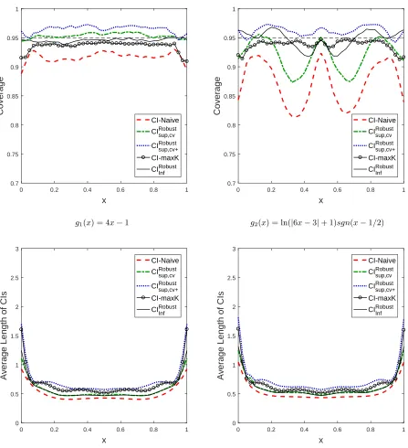
Figure 1 reports nominal 95% coverage probability and the length of CIs for “linear” and
“nonlinear” designs (g1(x) and g2(x)) using polynomials. Figure 2 displays results for “highly
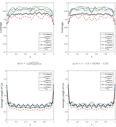
nonlinear” designs (g3(x) and g4(x)) using quadratic splines with a different number of knots.
Overall, we find (1) coverage of CIs based on theKb (e.g., selected by cross-validation or using more
terms than the cross-validation) using larger critical valuebc
sup
1−α(CIsup,cvRobust andCIsup,cv+Robust) is close to
or above 95%; (2) coverage of CI based on the infimum t-statistic (CIRobust
inf ) is close to the nominal
95% level and performs well across the different simulation designs. In terms of length, CIRobust inf
andCIRobust
sup,cv are quite similar and are narrower thanCImaxK (standard CI with undersmoothed K)
over the support. CINaive (using optimal MSE rate) has shortest length, but its coverage is far less
than 95% in many cases. Also note thatCIRobust
sup,cv+ is robust to specification search as well as bias
because it uses undersmoothedK, and thus length of CIRobust
sup,cv+ seems wide. However, coverage of
CIRobust
sup,cv+ is no less than 95% at almost all points in different setups.
For the linear function g1(x), finite sample bias is expected to be small overK∈ Kn as polyno-mials approximate unknown function well for allK. In this case, as theory predicted in Corollary 4.1, Figure 1 shows that coverage ofCIRobust
inf , CImaxK are close to the nominal 95% and coverage of
CIRobust
sup,cv, CIsup,cv+Robust are slightly above 95% for many points of the support. Given the small sample
size, coverage ofCIRobust
inf performs well even at the boundary and length is narrower thanCImaxK.
17
I also consider coverage of CI using the smallest number of series termsK, but it is omitted as its coverage is far below 95% at most points in nonlinear designs. In terms of coverage, CIRobust