Abstract—Visible Light Positioning (VLP) has become an essential candidate for high-accurate positioning; however, its positioning accuracy is usually degraded by the noise in the VLP system. To solve this problem, a novel scheme of noise measurement and mitigation is proposed for VLP based on the noise measurement from Allan Variance and the noise mitigation from positioning algorithms such as Adaptive Least Squares (ALSQ) and Extended Kalman Filter (EKF). In this scheme, Allan Variance is introduced for noise analysis in VLP for the first time, which provides an efficient method for measuring the white noise in the VLP systems. Meanwhile, we evaluate our noise reduction method under static test using ALSQ and dynamic test using EKF. Furthermore, this article carefully discusses the relationship between positioning accuracy and Dilution of Precision (DOP) values. The preliminary field static tests demonstrate that the proposed scheme improves the positioning accuracy by 16.5% and achieves the accuracy of 137 mm while dynamic tests show an improvement of 60.4% and achieve the mean positioning accuracy of 153 mm.
Index Terms—Visible Light Positioning (VLP), Allan Variance,
Adaptive Least Squares, Extended Kalman Filter, Navigation.
I. INTRODUCTION
ositioning service is now one of the essential technologies for social and scientific development. There have been several technologies to provide positioning services, such as Global Positioning System (GPS) [1], inertial sensors [2], Wireless Fidelity (WiFi) [3], Bluetooth [4], Radio-Frequency Identification (RFID) [5], Ultra Wideband (UWB) [6], Ultrasound [7], hybrid system [8], ZigBee [9], visible light [10], magnetic [11], geometry [12], and the integration of some of
these technologies [13, 14]. Meanwhile, many positioning algorithms such as trilateration [15], fingerprinting [16], and factor graph [17] have been widely used in the positioning systems. Among those technologies, Visible Light Positioning (VLP) has attracted the attention of many researchers in the past decade due to various technological breakthroughs in Visible Light Communication (VLC) technology, such as Light Fidelity (LiFi) [18]. Meanwhile, Light-Emitting Diode (LED) lamps, supporters for VLC, have become more and more popular in daily lives as energy-saving and environmentally-friendly lighting sources. VLC has many advantages over traditional wireless communication, including high data rate modulation, high energy efficiency, low heating, harmless to the human body, long lifetime, low maintenance cost [19] and so on. In addition, from the perspective of optical communication technology, since light cannot penetrate walls or ceilings, VLC systems in different rooms are independent and do not interfere with each other. From the perspective of positioning technology, since the visible light band is much larger than those radio waves such as microwave and millimeterwave, it is not interfered by various electromagnetic waves. When compared to signals such as WiFi and Bluetooth, visible light is not affected by severe multipath interference. Therefore, positioning technology based on visible light signals has great prospects.
In the past few years, many VLP algorithms have been proposed and verified through simulations and experiments, and the results show the positioning accuracy can reach centimeter-level in simulations and sub-meter-level in experiments [20-22]. In the industrial field, Philips, OSRAM, and Qualcomm have all launched their initial visible light indoor positioning solutions to work with smart devices to provide location services. However, the infrastructure has not become ready for large-scale VLP commercialization. Another main reason is that the VLP technology has not yet matured into the market. The VLP system is vulnerable to the external environment, which results in reduced stability in positioning performance [23]. Thus, it is essential to provide a reliable positioning solution that can deal with environmental noise for VLP applications.
The characteristics of the optical signals used in VLP bring a significant difference to positioning systems. These characteristics are Received Signal Strength (RSS), Time of Arrival (TOA), Time Difference of Arrival (TDOA), and Angle of Arrival (AOA). Among these characteristics, RSS is widely researched in VLP studies for its quick implementation and low computation complexity. Most RSS-based VLPs have achieved
Visible Light Positioning and Navigation Using
Noise Measurement and Mitigation
Yuan Zhuang, Member, IEEE, Luchi Hua, Qin Wang, Yue Cao, Member, IEEE, Zhouzheng Gao, Longning Qi, Jun Yang, Member, IEEE, and John Thompson, Fellow, IEEE
P
This work was supported by the National Natural Science Foundation of China under Grant 61771135, Grant 61574033 and Grant 41804027, the National Science and Technology Major Project of China under Grant 2017ZX01030101-002, and the Fundamental Research Funds for the Central Universities under Grant 2652018026. Copyright (c) 2015 IEEE. Personal use of this material is permitted. However, permission to use this material for any other purposes must be obtained from the IEEE by sending a request to [email protected].
Yuan Zhuang is with State Key Laboratory of Information Engineering in Surveying, Mapping and Remote Sensing, Wuhan University, 129 Luoyu Road, Wuhan 430079, China (email: [email protected]).
Luchi Hua, Qin Wang, Longning Qi and Jun Yang (corresponding author) are with Southeast University, 2 Sipailou, Nanjing 210096, China (e-mail: [email protected], [email protected], [email protected], [email protected]).
Yue Cao is with School of Computing and Communications, Lancaster University LA1 4WA, UK (e-mail: [email protected]).
Zhouzheng Gao is with School of Land Science and Technology, China University of Geosciences Beijing, 29 Xueyuan Road, Beijing, 100083, China (e-mail:[email protected]).
an accuracy of less than 0.5 m in simulations and field tests [20, 24, 25]. However, higher accuracy is demanded in some cases such as tracking goods on the pipeline, supervising robots and drones in the working field, and managing small assets.
To achieve higher accuracy, RSS-based VLPs need to improve the accuracy of the RSS measurements. RSS values are often affected by several factors including path loss, shadowing, multipath effect, which may change the RSS in the unit of dB. Noise is another big factor to affect the RSS in the unit of Watt. This paper focuses to mitigate the noise effects to improve the positioning accuracy of the VLP system. The noise effects in the VLP system are generated by not only the ambient signals but also the hardware of receiver and transmitter modules. Previous works show noise in VLP systems is mainly caused by shot noise and thermal noise [26]. Most studies analyze the influence of noise in VLP by simulations [26-29]. The study [28] determines the noise by measuring the background current with a specific instrument and then using the noise model. This specific instrument cannot always be found in the real-world environment. Some researches show that more disturbance might affect the RSS values in the practical environment, such as the perturbation of the illumination of the light source [23, 30]. However, shot noise and thermal noise are still main components in the VLP system [26, 31]. In summary, none of previous works has studied how to quickly measure the VLP noise without a specific instrument in the field environment and how to efficiently mitigate its influence.
Consequently, this article proposes a noise measurement and mitigation scheme to reduce the noise influence on the VLP system by introducing Allan Variance to noise measurement. Noise mitigation is performed with Adaptive Least Squares (ALSQ) and Extended Kalman Filter (EKF). Allan Variance is a time-domain-analysis technique that can be used to determine the characteristics of the data noise. It is a method of representing the Root Mean Square (RMS) random-drift errors as a function of averaging times [32]. Allan Variance has the advantages of directly measurable, simple to compute, and providing the types and magnitudes of various noise sources; thus, it is introduced as a tool to analyze the white noise (shot noise and thermal noise) and optical light fluctuation in the VLP system by processing the sampled sequence signal data from the receiver.
After the noise is analyzed by the Allan Variance, the next step is to find a method to efficiently mitigate the noise effects. In this article, we adopt ALSQ and EFK separately to cooperate with Allan Variance. Moreover, Dilution of Precision (DOP) is introduced as an indicator to demonstrate the positioning accuracy of the VLP system. The contributions of this article are summarized as follows.
[Noise Analysis for Visible Light Positioning Using Allan Variance] Previous VLP systems did not measure the noise directly or quickly. Thus, the Allan Variance is proposed for noise analysis in VLP for the first time, which provides a time-domain-analysis technique to directly and quickly determine the characteristics of noise effects in the VLP systems.
[ALSQ and EKF for Noise Mitigation in VLP] To reduce the noise influence on the positioning accuracy of the VLP system, ALSQ with a new convergence strategy based on the adaptive learning rate is proposed for VLP in static cases. The ALSQ considers the measured noise from Allan Variance in the estimation process by using it to update the observation covariance matrix. Meanwhile, the proposed new convergence strategy introduces an adaptive learning rate in the ALSQ to solve the divergence problem when using least squares for the non-linear model in the VLP system. For dynamic cases, EKF is proposed to estimate the receiver’s locations under the experimental environment. ALSQ and EKF efficiently mitigate the noise effects and improve the positioning accuracy for VLP in both static and dynamic cases.
The remainder of this article will be organized as follows: in Section II, a review of related works will be presented; in Section III, the methodology of this research will be discussed; in Section IV, this article will represent the test setup; in Section V, this article will discuss the results and analysis; finally, in Section VI, we will summarize our work.
II. RELATED WORK A. Allan Variance for Noise Analysis
Allan Variance was developed in the 1960s and initially applied in the clock system to study the frequency stability of oscillators [33]. It was then adopted to identify the error characteristics of inertial sensors [32]. That article gave the relationship between the Allan Variance and the Power Spectral Density (PSD) of different types of noises including quantization noise, bias instability, and Gaussian white noise. Published in 1999, the IEEE standard [34] included the process of analyzing inertial sensors with Allan Variance. In the 2000s, Allan Variance was proved to be a useful tool to study the error characteristics of Global Navigation Satellite System (GNSS) solutions [35]. In that article, first-order Gauss-Markov process, white noise, random walk, and flicker noise were identified as the dominant noise in the GNSS solutions by Allan Variance. Recently, Allan Variance was adopted to identify the colored noise, reflections, and shadowing from the wireless RSS values in wireless communication systems [36]. With Allan Variance, these noise effects were identified without considering the noise model or the complex spectral structure of the channel. B. Noise Analysis for Visible Light Systems
The noise sources, such as shot noise and thermal noise, can be found in any circuits involving p-n junctions [36], which are the components of photodiodes (PD). Therefore, how this noise affects the visible light system is an essential topic, which has been studied for decades. The shot noise in the P-I-N photodetector is generated by the LED light and ambient light. The thermal noise is caused by the operation of the amplifier and the load in the photodetector.
the noise model parameters on VLC systems. The research [28] explored the interference of different artificial lights on VLC. In this research, the noise was determined by measuring the background current on the PD. This work also studied how the noise affected the VLP. The study [29] simulated the positioning results for different noise types with various amplitudes. Simulation results illustrated that the average positioning error was 14.3 cm and 5.9 cm in a 4×4×6 m3 cell under direct and indirect sunlight exposure, respectively. In another research [37], the influence of the noise model parameters on VLP was investigated using the Cramer-Rao bound. Our previous work tried to use Allan variance to analyze the noise in the VLC systems [38].
C. RSS-based VLP with Disturbance Mitigation
RSS-based VLP systems with disturbance mitigation are found in works of literature [20, 24, 25, 39]. In the article [20], a RSS-distance model was established by considering the angle variation, distance variation, and light source variation. Coefficients were used to define the influence of specific light source group and light sensor. However, the dynamic variation of the signal and noises during localization are not considered. In the article [25], a carrier allocation method was proposed to mitigate the interferences between cells in the RSS-based VLP system, and then the trilateration method was used to calculate the coordinates. The study [39] used particle filter for positioning and consider the whole noise system as a non-Gaussian measurement noise. However, the study did not look into the noise characteristics in the system. Although some noise and disturbance can be non-Gaussian, the major noise should be particularly considered and verified. In the study [24], advanced filters were introduced to enable real-time tracking of the receiver. Kalman filter and particle filter can smooth positioning trail well when fine noise models are established. However, the study does not consider accurate noise and disturbance in the system rather depends on experience model and value of shot noise and thermal.
III. METHODOLOGY
The VLP performance is affected by white noise and other noises in the system. These noise effects are all random processes. In this article, a very convenient noise analysis method, the Allan Variance, is used to qualitatively analyze these noise sources. The Allan Variance directly observes different noise effects in the system and learns the noise coefficients for each noise source. However, as related articles have pointed out that the shot noise in the photoelectric sensor has the most significant influence on the signal in the visible light system and other noise sources (e.g., thermal noise) can be neglected [26, 31], it is unnecessary to consider all noise sources for noise mitigation in VLP. The shot noise can be modeled as Gaussian white noise, which has a specific curve characteristic in Allan Variance. Therefore, white noise in the VLP system will be quantitatively analyzed in this article. Then, ALSQ and EKF are proposed to mitigate the noise effects and further improve the positioning accuracy in two different cases (static and dynamic). Finally, ALSQ and EKF output the
positioning solutions. Moreover, ALSQ outputs the DOP of the positioning result.
A. System Structure
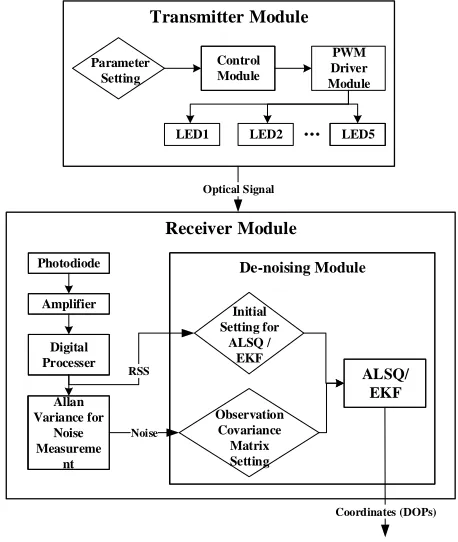
As shown in Fig. 1, the proposed VLP system mainly includes transmitter module and receiver module. The transmitter module configures the control parameters, which mainly include Pulse Width Modulation (PWM) waves-related parameters such as modulation frequency and duty cycle. Meanwhile, PD, amplifier, digital processor, noise measurement module, and noise mitigation module are included in the receiver module. The PD receives the optical signal from the transmitter module. The signal amplifier of the receiver module includes the inherent module circuit and external adjustment circuit. The digital processor performs the operations of windowing and Fast Fourier Transform (FFT) transformation and finally provides the received signal strength values corresponding to each LED. The received signal from the PD is processed by signal amplifier and digital processor and then sent to noise measurement module and noise mitigation module. The noise measurement module estimates the white noise through Allan Variance for each light source. The noise mitigation module obtains the noise information from the noise measurement module to update the observation covariance matrix, performs the modified least squares to process the observed light signals, and outputs the final positioning coordinates and its corresponding DOP value.
Receiver Module Transmitter Module
De-noising Module
PWM Driver Module
Control Module
LED5 LED2
LED1
Optical Signal
ALSQ/ EKF
Coordinates (DOPs)
Photodiode
Amplifier
Digital Processer
Initial Setting for
ALSQ / EKF
Observation Covariance Matrix Setting Parameter
Setting
RSS
Allan Variance for
Noise Measureme
nt
[image:3.612.324.553.374.645.2]Noise
Fig. 1. System structure of the proposed VLP system.
B. Allan Variance for Noise Measurement
measurements [36]. Instead, this article applies the Allan Variance method to the research field of VLP for the first time. The Allan Variance method can be explained as data instability in different sampling times. The specific principles are given as follows. Suppose there are Ns consecutive sampling data points, and the sampling interval is t0. The first step is to use
n
consecutive sampling points as a cluster (/ 2 s
nN ) and calculate the mean value of the cluster using
1 1, k n
k i
i k
x n x
n
(1) where k1, 2,...,n. The next step is to calculate the difference between every two adjacent data clusters, and the equation is
1, 1 .
k k xk n xk n
(2) The Allan Variance of a cluster with the length of T (T n t0 ) can be represented by
2 2
1,
1 . 2 k k T
(3)
That is
2 1
2 2
1 1
1
.
2 2 1
s N n
k k
k s
T x n x n
N n
(4)For a continuous random process, let us define its PSD as
X
S f . Then the relationship between the Allan Variance and the PSD is
4 2
2 0
sin
4 X fT d .
T S f f
fT
(5)According to IEEE standard [34], the Allan Variance for Gaussian white noise is given as
22
, N T
T
(6) where N represents the Gaussian white noise coefficient. The curve slope of the Allan Variance is 1/ 2 . The value of N is represented by
(1).
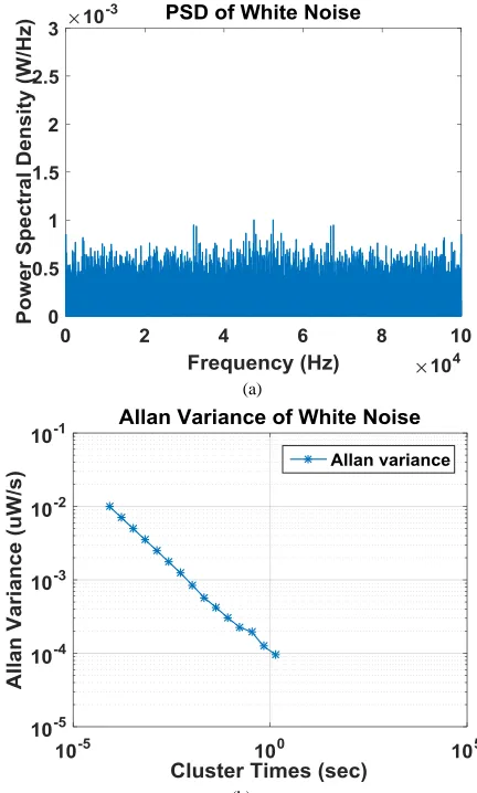
N (7) An illustration of the relationship between PSD and Allan Variance is shown in Fig. 2. The PSD of white noise is even distributed in its spectrum, which is shown in Fig. 2 (a). Based on Eq. (6), the log of is linear with the log of T; therefore, the blue line in Fig. 2 (b) has a linear trend.
The percentage error of the Allan Variance estimation for a specific cluster length T is expressed as
1. 2 Ns 1
n
(8)
The percentage error for cluster length of 1 second (n1) and 24 hours of sampled data (Ns 86400) is 0.24% while the percentage error becomes 9.21% for 1 minute of sampled data, which means the Allan Variance is more accurate when the sampling time is longer. The algorithm for noise measurement in the VLP system by using Allan Variance is summarized in Table I.
C. Positioning Algorithms with Noise Mitigation
After discussing the Allan Variance for noise measurement, this subsection starts to present the ALSQ and EKF for noise mitigation, which includes three parts: (I) ALSQ for positioning, (II) noise mitigation, and (III) EKF and Allan Variance. The first part will discuss how to design the ALSQ to process the RSS values from multiple LEDs to estimate the position of the receiver. The second part will present how to use the noise information, which is obtained from Allan Variance in the noise measurement module, to set the observation covariance matrix in the ALSQ to reduce the noise influence on positioning performance. The third part introduces how to cooperate noises from Allan Variance in EKF for visible light navigation.
(a)
[image:4.612.330.546.224.583.2](b)
Fig. 2. PSD and Allan Variance of white noise. (a) PSD and (b) Allan Variance.
TABLEI
THE ALGORITHM OF ALLAN VARIANCE FOR NOISE MEASUREMENT Input:
i
x : data sequence of the received optical signal from the receiver Output:
noise
: noise standard deviation from Allan Variance Process:
1. Calculate the mean value of cluster using Eq. (1); 2. Calculate the Allan Variance sequence using Eq. (4);
4. Output the noises with their coefficients from the Allan Variance (e.g., Eq. (7)).
[Part I. ALSQ for Positioning] In our system, an RSS-based trilateration method is adopted to estimate target locations. A typical solution for the trilateration method is the Nonlinear Least Squares (NLSQ). When using NLSQ, the PD channel model is used to represent the relationship between the state vector (the receiver’s 2D coordinates x
x y,
T ) and measurements (the RSS values Pi). Then, the design matrix H, measurement misclosure vector z , and observation covariance matrix R are determined for the NLSQ. Finally, with all these parameters, NLSQ estimates the state vector error and use it to update the state vector and obtain the receiver’s 2D coordinates.The PD channel model for the RSS-based VLP is given as [10]
2
1 cos cos
, 2 i i m M i i T i s
m AP T g
P
D
(9)
where Pi is the RSS value, Di is the distance between the th
i
LED and the receiver, A is the effective area of the photodetector, PTi is the transmit power of the
th
i LED, is the irradiance angle at the source and is the incidence angle at the receiver. Ts
and g
represent the gain of the optical filter and the gain of the concentrator, respectively. M represents the Lambertian order of the photodetector andm
i is the Lambertian order of the ith LED source.If the receiver is kept parallel to the transmitters’ plane (normally a ceiling), we have . Furthermore, if the vertical distance between the receiver and the transmitter is known, the cosine parts and Di can be replaced with the receiver’s 2D coordinates (
x
and y).There should be at least three observed LEDs for the receiver to estimate its position; therefore, there are multiple equations for VLP which are expressed as
1 2 1 11 1 1 2
1
2 2
2 2 2 2
2 2 cos cos sin , cos cos sin , ..., cos cos sin . n m M m M m M n n
n n n
n P C D P C D P C D (10)
where
1
2 i T i i s
m AP T g
C
represents the constant of
the th
i LED, and i represents the PWM duty cycle of the LED. Since the PD channel model is nonlinear, Eq. (10) can be solved by the NLSQ.
In the NLSQ, the design matrix is formed by the derivatives of the measurement model (PD channel model) with respect to the state vector (x
x y, T). Before establishing the designmatrix, the channel model is simplified from Eq. (9) to
2
2 2 bi,i i i i
P a xx yy h (11)
where
1
/ 2 ii s
m M
i i T
a m APT g h , and
2
/ 2i i
b m M , h is the vertical distance between the transmitter and the receiver. Then, the derivatives of the simplified channel model are given as
1
2 2 2
1
2 2 2
2 , 2 . i i
i i i
i
b
i i
i i i
i
b
i i
a b x x
P
x x x y y h
a b y y
P
y x x y y h
(12)
Finally, the design matrix is obtained by using Eq. (12) and expressed as 1 2 1 2 ... . ... T n n P P P
x x x
P
P P
y y y
H (13)
The measurement misclosure vector for the NLSQ is defined as
1 1 ˆ ˆ, 2 2 ˆ ˆ, ˆ ˆ, ,
T n n
P P x y P P x y P P x y
z (14)
where Pi is the observed RSS value, and P x yi
ˆ ˆ,
is the estimated RSS value, which is obtained by inputting the position estimate
x yˆ ˆ, to Eq. (11). Without knowing the noise characteristics of the received RSS values from the observed visible light, the observation covariance matrix (R matrix) of the NLSQ is usually set as, R C
R I (15) where CR represents the noise variance factor and I is the identity matrix.
Let xˆ
x yˆ ˆ,
T be the estimate of the state vector
x y,
T x and the estimated state vector error xˆ is represented by
ˆ ˆ
ˆ ˆ .
ˆ ˆ
dx x x
dy y y
x x x (16) ˆ
x can be calculated by using H matrix, the R matrix and the misclosure vector z as
1
1 1ˆ T T .
x H R H H R z (17)
Finally, the state vector is updated by using the xˆ as
1
ˆ k ˆ k ˆ.
x x x (18) The whole process of the NLSQ is an iterative process. Each cycle of the solution estimation consists of updating the design matrix H, misclosure vector z, state vector errorx,and state vector
x
. The cycle will end by achieve the pre-set maximum iterative cycles or state vector error threshold.NLSQ usually suffers from divergence problem. Therefore, we adopted ALSQ. Eq. (18) is changed as
1
ˆ k ˆk ˆ,
lr
where lr represents the adaptive learning rate. The H matrix in the new design is changed as follows
1 2 1 2 ... 1 . ... T n lr n P P P
x x x
P
P P
lr
y y y
H (20)
In the ALSQ, the convergence speed is controlled by lr, which is similar to the gradient descent method. A best choice of lr can maximize the convergence speed during the iteration. However, the best values for lr of all the locations on the map are not generally the same. Therefore, many self-adaptive lr strategies are proposed to address this issue. Our strategy is designed as follows
1 1 1
2 1 1
1 1
,
k k k
k k k k
k k k
lr lr lr lr z z z z z z (21)
where 1 and 2 are constants (11 and 21); is
2-norm. 11.3 and 20.7are set in our proposed system
based on practical experiments. Note that 1 and 2 should not
be too large or too small, and the initial lr should not be too large either. Fig. 3 shows the progress of the convergence of a selected location (location “24” as depicted in Fig. 7). A more clear view of the progress of the change of adaptive learning rate as the misclosure error changes is shown in Fig. 3 (b). The convergence ends fast at the 15th iteration.
[Part II. Noise Mitigation] A large positioning error in the NLSQ may be caused by the unknown noise characteristics of visible light, which indicates the importance of using Allan Variance to estimate the noises for the VLP system. Noise mitigation is another essential step to reduce the noise influence on positioning performance. With the noise obtained from Allan Variance, noise mitigation is easily implemented by setting the observation covariance matrix, R, in the NLSQ. The R matrix can be regarded as the variance of each noise disturbance in the system [40]. The variance of Gaussian white noise from each visible light has already been estimated by the Allan Variance. By assuming all visible lights are dependent from each other, the R matrix of the NLSQ can be expressed by these estimated variances as
2 2 2
1 2 ,
Tx Tx Txn
diag
R (22)
where 2
Txi
represents the noise variance from the ith LED and can be obtained by using the Allan Variance method. This resetting of the R matrix will improve the NLSQ to provide a more accurate position solution. Section V will show the positioning results before and after “noise measurement and mitigation”, which will clearly illustrate the improvement.
[Part III. EKF and Allan Variance] The Allan Variance can also cooperate with filtering techniques such as Kalman filter and particle filter, which are more favored in dynamic positioning. In this article, we adopt EKF in our dynamic test. The EKF compensates the disadvantage of Kalman filter in processing nonlinear systems. In EKF, the system is transformed by using Taylor series to obtain an approximate
linearization model.
(a)
[image:6.612.327.565.66.244.2](b)
Fig. 3. Convergence progress of the positioning algorithm with the adaptive learning rate. (a) Variation of the adaptive leaning rate and misclosure vector during positioning (b) Variation from the 5th iteration.
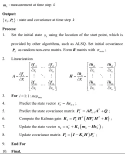
The observation covariance matrix, which is usually noted as R in the Kalman filter, is formed by the signal noise computed by Allan Variance. The process of EKF is shown in Table III. In Table II, A represents the state transfer matrix and H is the observation matrix. fs and ho represent nonlinear functions of state and observation. I represents the identity matrix.
TABLEII
EXTEND KALMAN FILTER ALGORITHM FOR NOISE MITIGATION Input:
sk1,Pk1: state and covariance at time step k1
k
m : measurement at time step k
Output:
sk,Pk: state and covariance at time step k
Process:
1. Set the initial state skusing the location of the start point, which is
provided by other algorithms, such as ALSQ. Set initial covariance k
P as random non-zero matrix. Form R matrix with noise; 2. Linearization 1 1 1 1 s s n s sn sn n x x X x x f f A f f f 1 1 1 1 o o n o on on n x x X x x h h h H h h
3. Fori1:1:stepnum
4. Predict the state vector k k1
s As ;
5. Predict the state covariance matrix 1
T
k k
P AP A Q;
6. Compute the Kalman gain T
T
k k k
K P H HP H R ;
7. Update the state vector k k k
k k
s s K m Hs ;
8. Update covariance matrix k k k
P I K H P ;
9. End For 10. Final.
D. Dilution of Precision
[image:6.612.314.564.396.710.2]of the Loran-C navigation system, can be used to show how range errors affect the positioning results [41]. A smaller DOP value usually illustrates a smaller positioning error. In RSS-based systems, the range errors mainly come from the measurement errors of RSS values. The proposed system aims to mitigate noise in RSS measurements to improve the positioning accuracy; therefore, DOP is a very useful approach to evaluate the system performance. The DOP has several flavors, such as: 1) Geometrical DOP (GDOP) [42], 2) Positional DOP (PDOP), 3) Horizontal DOP (HDOP), 4) Vertical DOP (VDOP), and 5) Time DOP (TDOP). HDOP was used in GPS to evaluate the horizontal positioning performance and defined as [41]
2 2
, E N
HDOP
(23) where
represents a standard deviation factor for all observations, which is the square root of the variance factor 2in Eq. (25); 2
E and 2
N
are the variances in the east and north directions. Similarly, we redefine the HDOP as follows for indoor VLP systems
2 2
, x y
HDOP
(24) where x2 and
2 y
are the variances of the x axis and y axis of the positioning coordinate frame (p-frame), in which the receiver position is estimated. The next step is to discuss the calculation of HDOP. From Eq. (17), the covariance matrix,
ˆ
x
P , of the estimated state vector xˆ can be given as
1 1 ˆ
1 2 1
1
2 1
, T
T T
x
R
R
P H R H
H Q H
H Q H
(25)
where
2 2 2 2 2 2
1/ 2/ ... /
Tx Tx Txn
diag
R
Q ; 2
is the variance factor. The diagonal elements of Pxˆ are the
estimated coordinate variances. By defining T 1
P R
Q H Q H,
P
Q can de described by
ˆ 2 .
x
P
P
Q (26) From Eq. (24) and (26), the HDOP follows
11 22.HDOP QP QP (27)
Finally, Eq. (27) is used to calculate the HDOP in the proposed system for performance analytics.
IV. TEST SETUP
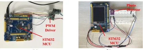
We set up a field test environment in Sensors Center, Southeast University, Wuxi, China, which included 5 LED lamps (Cree T6) and a PD receiver (OPT101), as shown in Fig. 4 (a). Each lamp was modulated by the PWM wave of the TIMER output of the STM32 Microcontroller Units (MCU), which is depicted in Fig. 5 (a). The frequencies of the LEDs were selected at 1.8 kHz, 2.572 kHz, 3.2 kHz, 4.5 kHz and 5.0
kHz, and the duty ratio was 70%.
Since the focus of this article is on noise measurement and mitigation for the VLP systems, multipath interference (light reflection), unstable external light interference, and other disturbance factors should be avoided as much as possible in the experiments. Therefore, according to the size of the test environment, a background cloth bracket with a size of 5×2.5m2 was hung to construct a darkroom environment. This black background cloth absorbed most of the lights that hit its surface; therefore, there were almost no reflected lights. Although there was no guarantee that the site was completely closed by the cloth bracket, the shielding of walls and window glass was ensured. The darkroom conditions could be satisfied since the experiments were conducted at night and the streetlights outside the window could not enter or affect the experimental environment.
The size of the experimental environment was 5×5×2.843 m3, which was a relatively large size for the field tests of current VLP systems and close to the sizes of most simulation environments [43, 44]. The uniform distribution of the LEDs, as shown in Fig. 4 (b), was similar to the real-world case, which ensured the natural extension to the large-scale deployment. The intervals among the LEDs were more than 2.8 m, which was a very sparse distribution and met the distributed spacing of most office LEDs. It was unnecessary to add additional LEDs between the existing ones that were used for lighting. Thus, the proposed VLP system was cost-efficient. However, positioning was more challenging under such a sparse distribution of source lights. In the experiment, the 10W LED single lamp was selected as the light source to save energy consumption. Meanwhile, the Texas Instruments OPT101 was selected as the photodetector in the receiver. The output of the photodetector was sent to the AD pins on the STM32 MCU, which is shown in Fig. 5 (b). An SD card was inserted in the board to store the data. Finally, parameter settings of the system environment are summarized in Table V.
[image:7.612.313.557.492.594.2](a) (b)
Fig. 4. Field setup of the VLP system. (a) General view of the system and (b) LED layout.
STM32 MCU
PWM Driver
Photo Detector
STM32 MCU
(a) (b)
[image:7.612.316.565.626.713.2]TABLEIII
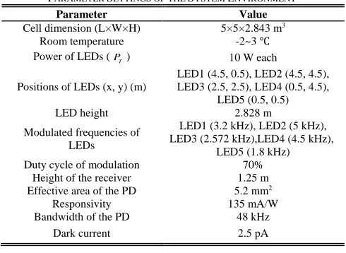
PARAMETER SETTINGS OF THE SYSTEM ENVIRONMENT
Parameter Value
Cell dimension (L×W×H) 5×5×2.843 m3
Room temperature -2~3 ℃
Power of LEDs (PT ) 10 W each
Positions of LEDs (x, y) (m)
LED1 (4.5, 0.5), LED2 (4.5, 4.5), LED3 (2.5, 2.5), LED4 (0.5, 4.5),
LED5 (0.5, 0.5)
LED height 2.828 m
Modulated frequencies of LEDs
LED1 (3.2 kHz), LED2 (5 kHz), LED3 (2.572 kHz),LED4 (4.5 kHz),
LED5 (1.8 kHz) Duty cycle of modulation 70%
Height of the receiver 1.25 m Effective area of the PD 5.2 mm2
Responsivity 135 mA/W
Bandwidth of the PD 48 kHz
Dark current 2.5 pA
V. RESULTS AND ANALYTICS A. Simulation Test
The parameters of the simulation environment are depicted in Table III. The optical signals received from each LED were simulated by using the PD channel model in Eq. (11) plus a random Gaussian white noise, whose noise variance was set by using the Allan Variance results in the field tests. The R matrix in the ALSQ was also generated by using these white noise variances. The positioning results before and after denoising (noise measurement and mitigation) are demonstrated in Fig. 6 and Table IV. Table IV depicts that the average positioning error was reduced by 25.5% and root mean square was reduced by 26.9% when using the denoising process. The Cumulative Distribution Function (CDF) in Fig. 6 shows that 50% and 90% positioning errors were improved by 21.1% and 18.3%, respectively.
TABLEIV
SIMULATED POSITIONING RESULTS (WITHOUT SYSTEM BIASES)
System Mean (m) RMS (m) 50% CDF (m)
90% CDF (m)
Before de-noising 0.051 0.067 0.038 0.104 After de-noising 0.038 0.049 0.030 0.085 Improvement 25.5% 26.9% 21.1% 18.3%
Fig. 6. Simulated 2D positioning results of 25 locations without system biases.
In this test, we also analyzed the relationship between DOP and positioning accuracy in the 25 tested locations which are marked in Fig. 6. The positioning process was simulated 60 times at each location. The simulation results are depicted in Fig. 7, where “MPE” stands for the “Mean Positioning Error” of the 60 positioning results. Fig. 7 illustrates that the positioning error was decreased after the denoising process and the DOP values stayed almost the same after the denoising process. Since the system noise were effectively measured and mitigated by Allan Variance and ALSQ, the positioning error become smaller. However, the denoising process did not significantly change the DOP values since DOP values were mainly affected by the geometry distribution of between the receiver and LEDs. In Fig. 7, both MPE and DOP values at the corner areas (locations of “1”, “5”, “21”, and “25”) were larger than other locations due to the poor geometry layout of the receiver and LEDs at the corner areas. Fig. 7 shows the DOP and MPE had the similar change trend. As the MPE was not always known when positioning in the real-world environment, DOP could be used as an efficient indicator to show the system positioning accuracy.
Fig. 7. DOP and MPE in the normal case (without simulated system biases). The box plot shows the interquartile ranges & outliers of the DOP values at each location. The red line represents the MPE at each location.
Typically, there are some unpredictable factors in the system and environment to affect the positioning performance in real-world environment. For example, the vertical distance may be different at various locations since the ceiling, and the floor are not always perfectly parallel. Another critical factor is the receiver’s gesture. Since many VLP systems are based on the assumption that receiver is kept horizontal during the positioning, a tilted angle of the receiver may cause a bias in the receiver signal and further affect the positioning accuracy. It is difficult to evaluate how these two factors affect the positioning performance in the field experiment. However, it can be easily assessed in the simulation, and therefore these two factors were studied in the simulation.
[image:8.612.51.296.75.254.2]were not significantly changed since DOP values were mainly affected by the geometry distribution of between the receiver and LEDs. The simulation results also depict that the denoise process reduced the mean and RMS of the positioning errors by 19.0% and 27.0%, respectively.
To learn how the tilted angle affects the positioning performance, a random angle bias with zero mean was added during the generation of the received optical signals in the simulation. The positioning results before and after de-noising are shown in Fig. 10, Fig. 11, and Table VI. The results demonstrate that the positioning accuracy was degraded significantly by the random tilted angle when compared with the normal case. Similar to the previous two simulations, the DOP values were not significantly changed by the random tilted angle. The simulation results also depict that the denoise process reduced the mean and RMS of the positioning errors by 28.0% and 34.4%, respectively. All these three simulations demonstrate that the proposed denoise process improved the positioning accuracy of the VLP system at different cases.
Although the Allan Variance method is first introduced in VLP, there are some noise reduction methods being widely used in other fields. Such as average filter [45], and wavelet de-noising [46]. The simulation results of these methods and our method are shown in Table VII and Fig. 12. In this simulation, the noises are composed by white noise and colored noise, which is simulated to stay close to the real-world environment. The positioning results in Fig. 12 (a) show that the estimated locations by Allan Variance are uniformly close to the physical locations. The same conclusion also can be seen in Fig. 12 (b). Table VII shows that the wavelet de-noising outperforms the average filter while Allan Variance provides the best performance in most indicators. The improvements of the average filter, wavelet de-noising, and Allan Variance are 11.43%, 17.14%, and 30.0%.
Fig. 8. Simulated 2D positioning results of 25 locations with random height error.
TABLE V
SIMULATED POSITIONING RESULTS (WITH RANDOM HEIGHT ERROR)
System Mean (m) RMS (m) 50% CDF (m)
90% CDF (m)
[image:9.612.320.563.59.212.2]Before de-noising 0.116 0.159 0.084 0.210 After de-noising 0.094 0.116 0.074 0.167 Improvement 19.0% 27.0% 11.9% 20.5%
[image:9.612.325.545.258.418.2]Fig. 9. DOP and MPE in the case of simulated random height error. The box plot shows the interquartile ranges & outliers of the DOP values at each location. The red line represents the MPE at each location.
Fig. 10. Simulated 2D positioning results of 25 locations with random titled angle.
TABLE VI
SIMULATED POSITIONING RESULTS (RANDOM TILTED ANGLE)
System Mean (m) RMS (m) 50% CDF (m)
90% CDF (m)
[image:9.612.317.567.471.704.2]Before de-noising 0.125 0.163 0.094 0.249 After de-noising 0.090 0.107 0.082 0.118 Improvement 28.0% 34.4% 12.8% 52.6%
[image:9.612.52.299.689.739.2](a) (b)
Fig. 12. Simulated positioning results of Allan Variance and other noise reduction methods. (a) 2D positioning results of 25 locations, (b) The CDFs of the positioning errors.
TABLE VII
POSITIONING RESULTS OF ALLAN VARIANCE AND OTHER METHODS
System Mean (m) RMS (m) 50% CDF (m)
90% CDF (m)
Before de-noising 0.070 0.114 0.040 0.198 Average filter 0.062 0.093 0.045 0.329 Wavelet 0.058 0.090 0.035 0.153 Allan Variance 0.049 0.079 0.038 0.076
B. Field Test a. Static Test
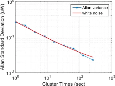
The parameters for the field test are shown in Table III. The Allan Variance of the signals received from each LED was analyzed individually. During the test, there was only one LED turned on and no ambient light (in the darkroom). The result of Allan Variance is illustrated in Fig. 13. Note that the red line which stands for the Gaussian white noise fits the left half of the Allan Variance curve by using least squares to minimize the fitting error.
To evaluate the performance of the proposed VLP system, a total of 25 locations were collected in the darkroom, and the RSS values at each location were collected for 18 times. These
RSS values were substituted into the ALSQ as the measurement vector. The positioning results before the noise mitigation are shown in Fig. 14 (a) and Fig. 14 (b). It demonstrates that the positioning results at the edge area were far from the ground truth, which might be caused by the low SNR at the edge area and the poor geometry layout of the receiver and LEDs. Fig. 14 (d) shows the CDF of the positioning error. The results showed that 90% and average positioning errors were 0.315 m and 0.164 m, respectively.
Fig. 13. Allan Variance of the RSS values received from one LED (5 kHz) under the conditions of only one LED on and no ambient light interference.
For the same data in the field tests, the positioning results after noise mitigation are demonstrated in Fig. 14 (a) and Fig. 14 (c). The results showed that the average positioning error after noise mitigation was 0.137 m; therefore, the positioning accuracy was improved by 16.5% by the noise mitigation. As shown in Fig. 14 (d), 90% positioning error after noise mitigation was 0.267 m, which had 15.2% improvement when compared to the positioning results before noise mitigation.
(a) (b) (c)
[image:10.612.53.297.53.159.2](d) (e) (f)
[image:10.612.346.532.168.308.2] [image:10.612.49.564.445.694.2]Fig. 14 (d) and Table VIII illustrate that most of the positioning errors were reduced by the noise mitigation process. The DOP values at 25 locations before and after mitigation are shown in Fig. 14 (e) and Fig. 14 (f). Similar to the simulation, both MPE and DOP values at the corner areas (locations of “1”, “5”, “21”, and “25”) were larger than other places due to the poor geometry layout of the receiver and LEDs at the corner areas. Fig. 14 (e) and Fig. 14 (f) showed the DOP and MPE had the similar change trend for most of the time.
To compare the proposed VLP system with previous related works, we summarize their differences in Table IX. “TRI” in Table IX represents the “trilateration” method, and “Sim/Exp” stands for “simulation/experiment”. In Table IX, simulations have better positioning results than field experiences as they cannot consider all the factors which affect the positioning performance in the real-world environment. During all the field experiments, the proposed VLP system achieves the highest accuracy (14 cm), which is equal to the system proposed in [47]. However, the system in [47] was tested in a small area and aided by inertial sensors. Overall, the proposed VLP system achieves an impressive positioning accuracy by only using a PD as the receiver.
TABLEVIII
POSITIONING RESULTS BEFORE AND AFTER DE-NOISING
System Mean (m) RMS (m) 50% CDF (m)
90% CDF (m)
Before de-noising 0.164 0.191 0.152 0.315 After de-noising 0.137 0.166 0.110 0.267 Improvement 16.5% 13.1% 27.6% 15.2% b. Dynamic Test
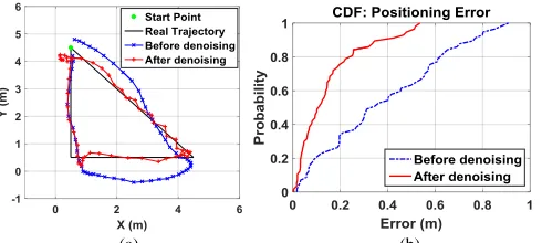
We performed a dynamic test under the same environment. The receiver was hold horizontally at 1.593 m and moved along a triangle trajectory clockwise as shown in Fig. 15 (a). It started at (4.5 m, 4.5 m), moving towards (4.5 m, 0.5 m). The moving speed was 1 m/s constantly. Estimated Position was computed every 0.5 s using EKF.
[image:11.612.53.298.482.592.2](a) (b)
Fig. 15. Positioning results of the receiver moving along a triangle trajectory using EKF with and without denoising. (a) 2D Positioning results, (b) CDF of the positioning results.
TABLEIX
COMPARISON BETWEEN RELATED WORKS AND OURS
Cell size Principle Accuracy
[25] 0.6m×0.6m×0.6m TRI 3D: 24 mm (Sim) [24] 6m×6m×4.2m TRI+PF/KF 2D: <150 mm (Sim) [47] 2.5m×2.8m×2.5m TRI+PDR+PF 2D: 140 mm (Exp)
[20] 5m×8m TRI 2D: 300 mm (Exp)
Ours 5m×5m×2.8m
TRI (Allan Variance+ALSQ)
EKF+Allan Variance
2D: 137 mm (Exp) 2D: 153 mm (Exp)
Fig. 15 (a) shows the positioning results of the dynamic test. In Fig. 15 (a), trajectory in blue was generated by EKF with R matrix set as identity matrix. Trajectory in red was generated by EKF with R matrix formed by Allan Variance results. This figure shows that the EKF method with denoising is much closer to the real trajectory than the EKF without denoising. Fig. 15 (b) indicates that by cooperating noises from Allan Variance in EKF, positioning performance is well improved. The average positioning error of EKF with denoising was 0.153 m, while EKF without denoising was 0.386 m, indicating an improvement of 60.4%.
VI. CONCLUSION AND FUTURE WORK
A novel scheme of noise measurement and mitigation was proposed for VLP based on noise measurement from Allan Variance and noise mitigation from ALSQ and EKF. The DOP value was used as an indicator to show the positioning accuracy of the VLP system. Simulation results illustrated that the proposed VLP system achieved the average positioning accuracy of 38 mm, which had 25.5% improvement when compared with the conventional scheme. With simulated random height error and random titled angle, the average positioning accuracy still had the improvement of 19.0% and 28%, respectively. Conventional de-noising methods including average filtering and wavelet de-noising were investigated and compared with Allan Variance. Simulation results indicated that Allan Variance provides better performance than these methods in VLP. The field static tests showed that the proposed VLP system achieved the positioning accuracy of 137 mm with the improvement of 16.5%. The field dynamic tests showed that EKF using Allan Variance method improved positioning performance by 60.4%. These results demonstrated that Allan Variance was an efficient method to measure noises for VLP. Both simulation and field tests showed DOP was an efficient indicator to depict the positioning accuracy. The results showed both positioning errors and DOP values at the corner areas are larger than the center area. We will continue to evaluate the performance of our proposed VLP system by comparing it with related works in a large-scale environment.
REFERENCES
[1] H. Liu, S. Nassar, and N. El-Sheimy, "Two-filter smoothing for accurate INS/GPS land-vehicle navigation in urban centers," IEEE Transactions on Vehicular Technology, vol. 59, pp. 4256-4267, 2010.
[2] R. Harle, "A survey of indoor inertial positioning systems for pedestrians," IEEE Communications Surveys and Tutorials, vol. 15, pp. 1281-1293, 2013.
[3] Y. Zhuang, Z. Syed, Y. Li, and N. El-Sheimy, "Evaluation of two WiFi positioning systems based on autonomous crowdsourcing of handheld devices for indoor navigation," IEEE Transactions on Mobile Computing, vol. 15, pp. 1982-1995, 2016.
[4] Y. Zhuang, J. Yang, Y. Li, L. Qi, and N. El-Sheimy, "Smartphone-Based Indoor Localization with Bluetooth Low Energy Beacons," Sensors, vol. 16, p. 596, 2016.
[5] A. R. J. Ruiz, F. S. Granja, J. C. P. Honorato, and J. I. G. Rosas, "Accurate pedestrian indoor navigation by tightly coupling foot-mounted IMU and RFID measurements," IEEE Transactions on Instrumentation and measurement, vol. 61, pp. 178-189, 2012.
round-trip-time measurements," IEEE Transactions on Intelligent Transportation Systems, vol. 17, pp. 2272-2281, 2016.
[7] Z. Farid, R. Nordin, and M. Ismail, "Recent advances in wireless indoor localization techniques and system," Journal of Computer Networks and Communications, vol. 2013, 2013.
[8] N. Alam and A. G. Dempster, "Cooperative positioning for vehicular networks: Facts and future," IEEE Transactions on Intelligent Transportation Systems, vol. 14, pp. 1708-1717, 2013.
[9] S.-H. Fang, C.-H. Wang, T.-Y. Huang, C.-H. Yang, and Y.-S. Chen, "An enhanced zigbee indoor positioning system with an ensemble approach," IEEE Communications Letters, vol. 16, pp. 564-567, 2012.
[10] Y. Zhuang, L. Hua, L. Qi, J. Yang, P. Cao, Y. Cao, et al., "A Survey of Positioning Systems Using Visible LED Lights," IEEE Communications Surveys & Tutorials, vol. 20, pp. 1963-1988, 2018.
[11] Y. Li, Y. Zhuang, H. Lan, P. Zhang, X. Niu, and N. El-Sheimy, "Self-contained indoor pedestrian navigation using smartphone sensors and magnetic features," IEEE Sensors Journal, vol. 16, pp. 7173-7182, 2016. [12] O. Kaiwartya, Y. Cao, J. Lloret, S. Kumar, N. Aslam, R. Kharel, et al., "Geometry-Based Localization for GPS Outage in Vehicular Cyber Physical Systems," IEEE Transactions on Vehicular Technology, vol. 67, pp. 3800-3812, 2018.
[13] Y. Zhuang and N. El-Sheimy, "Tightly-coupled integration of WiFi and MEMS sensors on handheld devices for indoor pedestrian navigation," IEEE Sensors Journal, vol. 16, pp. 224-234, 2016.
[14] Y. Li, Y. Zhuang, P. Zhang, H. Lan, X. Niu, and N. El-Sheimy, "An improved inertial/wifi/magnetic fusion structure for indoor navigation," Information Fusion, vol. 34, pp. 101-119, 2017.
[15] B. T. Fang, "Trilateration and extension to global positioning system navigation," Journal of Guidance, Control, and Dynamics, vol. 9, pp. 715-717, 1986.
[16] K. Kaemarungsi and P. Krishnamurthy, "Modeling of indoor positioning systems based on location fingerprinting," in Ieee Infocom 2004, 2004, pp. 1012-1022.
[17] C. Mensing and S. Plass, "Positioning based on factor graphs," EURASIP Journal on Advances in Signal Processing, vol. 2007, p. 041348, 2007. [18] H. Haas, L. Yin, Y. Wang, and C. Chen, "What is lifi?," Journal of
Lightwave Technology, vol. 34, pp. 1533-1544, 2016.
[19] A. Sevincer, A. Bhattarai, M. Bilgi, M. Yuksel, and N. Pala, "LIGHTNETs: Smart LIGHTing and mobile optical wireless NETworks—A survey," IEEE Communications Surveys & Tutorials, vol. 15, pp. 1620-1641, 2013.
[20] L. Li, P. Hu, C. Peng, G. Shen, and F. Zhao, "Epsilon: A Visible Light Based Positioning System," in NSDI, 2014, pp. 331-343.
[21] Y. Zhuang, Q. Wang, M. Shi, P. Cao, L. Qi, and J. Yang, "Low-Cost Localization for Indoor Mobile Robots Based on Ensemble Kalman Smoother Using Received Signal Strength " IEEE Internet of Things Journal 2019.
[22] Y. Zhuang, Q. Wang, Y. Li, Z. Gao, B. Zhou, L. Qi, et al., "The Integration of Photodiode and Camera for Visible Light Positioning by Using Fixed-Lag Ensemble Kalman Smoother," Remote Sensing, vol. 11, p. 1387, 2019.
[23] Y. Zhang, Y. Zhu, W. Xia, F. Yan, L. Shen, and Y. Wu, "Localization for visible light communication with practical non-Gaussian noise model," in Wireless Communications and Signal Processing (WCSP), 2017 9th International Conference on, 2017, pp. 1-6.
[24] W. Gu, W. Zhang, M. Kavehrad, and L. Feng, "Three-dimensional light positioning algorithm with filtering techniques for indoor environments," Optical Engineering, vol. 53, pp. 107107-107107, 2014.
[25] H.-S. Kim, D.-R. Kim, S.-H. Yang, Y.-H. Son, and S.-K. Han, "An indoor visible light communication positioning system using a RF carrier allocation technique," Journal of Lightwave Technology, vol. 31, pp. 134-144, 2013.
[26] T. Komine and M. Nakagawa, "Fundamental analysis for visible-light communication system using LED lights," IEEE transactions on Consumer Electronics, vol. 50, pp. 100-107, 2004.
[27] F. Madani, G. Baghersalimi, and Z. Ghassemlooy, "Effect of transmitter and receiver parameters on the output signal to noise ratio in visible light communications," in Electrical Engineering (ICEE), 2017 Iranian Conference on, 2017, pp. 2111-2116.
[28] A. J. Moreira, R. T. Valadas, and A. de Oliveira Duarte, "Optical interference produced by artificial light," Wireless Networks, vol. 3, pp. 131-140, 1997.
[29] W. Zhang, M. S. Chowdhury, and M. Kavehrad, "Asynchronous indoor positioning system based on visible light communications," Optical Engineering, vol. 53, pp. 045105-045105, 2014.
[30] E. Giard, B. L. Nghiem, M. Caes, M. Tauvy, I. Ribet-Mohamed, R. Taalat, et al., "Noise measurements for the performance analysis of infrared photodetectors," in 2013 22nd International Conference on Noise and Fluctuations (ICNF), 2013, pp. 1-4.
[31] P. Lou, H. Zhang, X. Zhang, M. Yao, and Z. Xu, "Fundamental analysis for indoor visible light positioning system," in Communications in China Workshops (ICCC), 2012 1st IEEE International Conference on, 2012, pp. 59-63.
[32] N. El-Sheimy, H. Hou, and X. Niu, "Analysis and modeling of inertial sensors using Allan variance," IEEE Transactions on instrumentation and measurement, vol. 57, pp. 140-149, 2008.
[33] D. W. Allan, "Statistics of atomic frequency standards," Proceedings of the IEEE, vol. 54, pp. 221-230, 1966.
[34] N. Single-Axis, "IEEE Standard Specification Format Guide and Test Procedure for Linear," 1999.
[35] X. Niu, Q. Chen, Q. Zhang, H. Zhang, J. Niu, K. Chen, et al., "Using Allan variance to analyze the error characteristics of GNSS positioning," GPS solutions, vol. 18, pp. 231-242, 2014.
[36] C. Luo, P. Casaseca-de-la-Higuera, S. McClean, G. Parr, and P. Ren, "Characterisation of Received Signal Strength Perturbations using Allan Variance," IEEE Transactions on Aerospace and Electronic Systems, 2017.
[37] X. Zhang, J. Duan, Y. Fu, and A. Shi, "Theoretical accuracy analysis of indoor visible light communication positioning system based on received signal strength indicator," Journal of Lightwave Technology, vol. 32, pp. 3578-3584, 2014.
[38] L. Hua, Y. Zhuang, L. Qi, J. Yang, and L. Shi, "Noise Analysis and Modeling in Visible Light Communication Using Allan Variance," IEEE Access, vol. 6, pp. 74320-74327, 2018.
[39] D. Zheng, K. Cui, B. Bai, G. Chen, and J. A. Farrell, "Indoor localization based on LEDs," in Control Applications (CCA), 2011 IEEE International Conference on, 2011, pp. 573-578.
[40] J. J. Sudano, "A least square algorithm with covariance weighting for computing the translational and rotational errors between two radar sites," in Aerospace and Electronics Conference, 1993. NAECON 1993., Proceedings of the IEEE 1993 National, 1993, pp. 383-387.
[41] R. B. Langley, "Dilution of precision," GPS world, vol. 10, pp. 52-59, 1999.
[42] I. Sharp, K. Yu, and Y. J. Guo, "GDOP analysis for positioning system design," IEEE Transactions on Vehicular Technology, vol. 58, pp. 3371-3382, 2009.
[43] A. Taparugssanagorn, S. Siwamogsatham, and C. Pomalaza-Ráez, "A hexagonal coverage LED-ID indoor positioning based on TDOA with extended Kalman filter," in Computer Software and Applications Conference (COMPSAC), 2013 IEEE 37th Annual, 2013, pp. 742-747. [44] T.-H. Do, J. Hwang, and M. Yoo, "TDoA based indoor visible light
positioning systems," in Ubiquitous and Future Networks (ICUFN), 2013 Fifth International Conference on, 2013, pp. 456-458.
[45] J. So, J.-Y. Lee, C.-H. Yoon, and H. Park, "An improved location estimation method for wifi fingerprint-based indoor localization," International Journal of Software Engineering and Its Applications, vol. 7, pp. 77-86, 2013.
[46] M. R. Mosavi and I. EmamGholipour, "De-noising of GPS receivers positioning data using wavelet transform and bilateral filtering," Wireless personal communications, vol. 71, pp. 2295-2312, 2013.
[47] Z. Li, A. Yang, H. Lv, L. Feng, and W. Song, "Fusion of visible light indoor positioning and inertial navigation based on particle filter," IEEE Photonics Journal, vol. 9, pp. 1-13, 2017.