Asymptotics and Well Posedness of the Derived Distribution Density in a Study of Biovariability

ISSN Online: 2152-7393 ISSN Print: 2152-7385

DOI: 10.4236/am.2018.96046 Jun. 28, 2018 672 Applied Mathematics

Asymptotics and Well-Posedness of the Derived

Distribution Density in a Study of Biovariability

Hongyun Wang

1

_{, Wesley A. Burgei}

2

_{, Hong Zhou}

3

1_{Department of Applied Mathematics and Statistics, University of California, Santa Cruz, CA, USA}

2_{US Department of Defense, Joint Non-Lethal Weapons Directorate, Quantico, VA, USA}

3_{Department of Applied Mathematics, Naval Postgraduate School, Monterey, CA, USA}

Abstract

In our recent work (Wang, Burgei, and Zhou, 2018) we studied the hearing loss injury among subjects in a crowd with a wide spectrum of heterogeneous individual injury susceptibility due to biovariability. The injury risk of a crowd is defined as the average fraction of injured. We examined mathemat-ically the injury risk of a crowd vs the number of acoustic impulses the crowd is exposed to, under the assumption that all impulses act independently in causing injury regardless of whether one is preceded by another. We con-cluded that the observed dose-response relation can be explained solely on the basis of biovariability in the form of heterogeneous susceptibility. We de-rived an analytical solution for the distribution density of injury susceptibili-ty, as a power series expansion in terms of scaled log individual non-injury probability. While theoretically the power series converges for all argument values, in practical computations with IEEE double precision, at large argu-ment values, the numerical accuracy of the power series summation is com-pletely wiped out by the accumulation of round-off errors. In this study, we derive a general asymptotic approximation at large argument values, for the distribution density. The combination of the power series and the asymptot-ics provides a practical numerical tool for computing the distribution densi-ty. We then use this tool to verify numerically that the distribution obtained in our previous theoretical study is indeed a proper density. In addition, we will also develop a very efficient and accurate Pade approximation for the distribution density.

Keywords

Distribution of Individual Injury Susceptibility in a Crowd, Biovariability, Asymptotic Approximation, Pade Approximation

How to cite this paper: Wang, H.Y., Bur-gei, W.A. and Zhou, H. (2018) Asymptotics and Well-Posedness of the Derived Distri-bution Density in a Study of Biovariability. Applied Mathematics, 9, 672-690. https://doi.org/10.4236/am.2018.96046

Received: May 3, 2018 Accepted: June 25, 2018 Published: June 28, 2018

Copyright © 2018 by authors and Scientific Research Publishing Inc. This work is licensed under the Creative Commons Attribution International License (CC BY 4.0).

http://creativecommons.org/licenses/by/4.0/

DOI: 10.4236/am.2018.96046 673 Applied Mathematics

1. Introduction

Sound is an indispensable part of our life and we experience sound every day. A common way to measure the amount of sound is the decibel (dB) [1]. Sounds of less than 75 dB are at safe levels that do not damage our hearing. However, any sound above 85 dB is potentially harmful and can cause hearing loss. Examples of harmless sounds are normal conversation (60 dB), the humming of a refrige-rator (45 dB) whereas harmful sounds include noise from lawn mowers (90 dB) and gun shots or firecrackers (both 150 dB) [2]. The risk of hearing damage de-pends on the power of the sound as well as the length of exposure.

Hearing loss is a common health problem among veterans. In order to protect warfighters, starting 1960s the US Army conducted and funded research to as-sess the risk of hearing loss caused by intense impulse noise from explosive blasts and weapon firings [3]. Recently Dr. Chan and his collaborators [4] de-veloped a dose-response model for the assessment of injury caused by impulse noise and a model for the possible recovery afterwards, based on chinchilla data. Chinchillas share similar hearing capabilities as humans and thereby are com-monly used for hearing-related experiments.

In [5], we interpreted the empirical dose-response relation from [4] for expo-sure to multiple sound impulses in the framework of immunity. In [6], we viewed the empirical dose-response relation from a completely different angle, in the framework of biovariability. Together in these two studies [5] [6], we showed that it is possible to interpret the empirical dose-response relation from either of the two extreme cases: immunity or biovariability. Here we would like to further our study in [6] to demonstrate that the derived distribution density of injury susceptibility in [6] is well-posed.

2. Mathematical Formulation of the Problem

In experiments [4], the injury risk of a crowd caused by a sound exposure event is described by the logistic dose-response relation:

(

)

(

50

)

1 1 exp

p

SELA D α

=

+ − − . (1)

Here the dose of the sound exposure event is defined by the SELA (A-Weighted Sound Exposure Level) in units of dBA. The injury risk p of the crowd represents the average injury fraction of the crowd. In the logistic dose response model (1), the parameter α determines the steepness of function p

DOI: 10.4236/am.2018.96046 674 Applied Mathematics

that the parameter value α remains unchanged (α =0.1_{) for PTS injuries of all}

cut-off levels whereas the median injury dose D50 rises with the PTS cut-off level

[4].

In the framework of the logistic dose-response relation, the injury risk of the crowd caused by a sequence of N acoustic impulses is given by the expression

( impulses)

(

₍

₎

)

comb 50

1 1 exp

N p

S D

α

=

+ − − . (2)

where Scomb is the effective combined dose for the whole sequence of impulses

as a single sound exposure event. For a sequence of N identical impulses each with SELA value S, the effective combined dose, Scomb, was observed to follow

the dose combination rule [4]:

comb log10 , 3.44

S = +S λ N λ= . (3) Thus, for a sequence of N impulses each with SELA value S, the injury risk takes the form

( impulses)

(

₍

₎

)

_{( )}

1 50 10

1 1

1 exp log ₁

N

p

S D N _aNη

α λ −

= ≡

+ − − + ₊ . (4)

where parameters a and η are defined as

(

)

(

50

)

exp , 0.1494

ln10

a≡ α S D− η≡ αλ = _{. (5)}

Parameter a is related to probability p_{(1 impulse)} by

(1impulse) (1impulse)

| =

1 |

p a

p

− . (6)

That is, parameter a is the injury odds of a hypothetical subject in the crowd with the average injury probability, p_{(1 impulse)}, in responding to a single acoustic impulse.

In [6] under the assumption that N acoustic impulses act independently from each other in causing injury, regardless of whether one is preceded by another (i.e., no immunity effect), we explored the possibility of interpreting the ob-served logistic dose-response relation for a crowd in the framework of biovaria-bility. For mathematical convenience, we consider non-injury probability in-stead of injury probability. Let q

( )

ω

_{denote the individual non-injury}

proba-bility of a random subject in the crowd, in responding to one acoustic impulse. Here q

( )

ω

_{is a random variable, due to the presence of biovariability. Let}

( )

q

ρ

_{be the distribution density of random variable} q

( )

ω

_{. Mathematically in}

the framework of biovariability, the average non-injury fraction for N acoustic impulses is expressed in terms of

ρ

( )

q as

(

)

_{( )}

( )

1

( )

impulses 0

Non-injury fraction N N d

frac-DOI: 10.4236/am.2018.96046 675 Applied Mathematics

tion as

(

)

_{( ) ( )}

( )

1

impulses impulses

1 1

Non-injury fraction 1 1

1 1

N

N p _aN

aNη − η

= − = − =

+

+ . (8)

For the theoretical model of biovariability to reproduce the experimentally observed results, the distribution density

ρ

( )

q has to satisfy an equation ob-tained by combining (7) and (8), which we write out below:

( )

1 0

1

d , 1,2,

1

N

q q q N

aNη

ρ = =

+

∫

. (9)

In [6] we solved Equation (9) analytically by constructing a power series

expansion in new variable

( )

1

ln

s aη q

−

= − . Since the non-injury probability

( )

q

ω

is constrained to interval

( )

0,1 , variable

( )

1

ln

s aη q

−

= − _{has the domain}

(

0,+∞

)

_{. The distribution density of random variable} s

( )

_ω aη1ln

(

q

( )

_ω

)

−

= − _is

( )

1 exp 1 exp 1

g s _≡aη_ρ _₋a sη __ _−a sη _

   

 _{ } _{ }

  . (10)

For density g s

( )

, Equation (9) becomes

( )

1

0 1

1

exp d

1 a N s g s s

a N η

η η

+∞    

−_ _  =

 _{ }  _{ }

  _{+  }

 

 

∫

. (11)

In [6] we derived a power series solution for g s

( )

:

( )

₍

( )

₍

₎

₎

( )1 1

0

1 1

k k k

g s s

k η η

+∞

+ −

= − =

Γ +

∑

. (12)

In power series (12), the gamma function Γ

(

η

(

k+1

)

)

_{in the denominator of}

the coefficient grows faster than any exponential function of k. As a result, pow-er spow-eries (12) convpow-erges for all values of s. It follows that function g s

( )

is well defined by power series (12) for all values of s. To be a proper density function, however, g s

( )

must satisfy the two properties below:

( )

0

g s ≥ (13)

( )

0 g s sd 1

+∞

=

∫

. (14)

In [6] we rigorously proved these two properties for the special case of η=1₂

and the special case of 1

3

η= _{. The analysis procedure differs quite significantly}

DOI: 10.4236/am.2018.96046 676 Applied Mathematics

we need the numerical capability of calculating function g s

( )

for all values of

s, from small to large. Power series (12) has the nice property that theoretically it converges for all values of s. In practical computations, however, at large values of s, the numerical accuracy of the power series summation is completely wiped out by the accumulation of round-off errors. In the power series summation, as s

increases the net sum decreases while the magnitude of the largest term grows exponentially with s[6]. The combined effect of these two factors magnifies ca-tastrophically, at large s, the influence of round-off errors on the numerical ac-curacy of the net sum. For practical computation of g s

( )

in finite precision arithmetic, we need a robust numerical formula of g s

( )

at large s. In the next section, we derive a general asymptotic approximation of g s

( )

at large s. The synthesis of the power series and the asymptotics will provide a practical nu-merical tool for computing the distribution density g s

( )

for all values of s at any given value of parameter η.

3. Asymptotics of

g

(

s

) at Large

s

Now we derive a general asymptotic approximation of g s

( )

at large s when η

is a rational number. We then reasonably conjecture that the same asymptotic approximation is also valid even when η is irrational. In practical computation of

( )

g s , the case of irrational η actually does not apply since all numerical calcula-tions are carried out in finite precision arithmetic, using only rational numbers.

A rational number η takes the form m n

η= _{where both m and n are positive}

integers. We rewrite the power series of g s

( )

in terms of the reciprocal gamma function as follows:

( )

( )

(

)

( )1 1

0 1 1

m k

k _n

k

m

g s f k s

n

+∞ _{+ −}

=

 

= − _ + _

 

∑

(15)

where f z

( )

is the reciprocal gamma function defined as

( )

_{( )}

1

f z z

≡

Γ . (16)

The advantage of working with the reciprocal gamma function f z

( )

is that it is well defined and is analytic everywhere. In comparison, the gamma function

( )

z

Γ diverges at all non-positive integer values of z. The reciprocal gamma function f z

( )

has the property

(

1

) ( )

_{( )}

1

₍

1

₎

(

1

)

1

z

z f z f z

z z

−

− = = = −

Γ Γ − . (17)

Using this convenient property when differentiating g s

( )

, we have

( )

( )

(

)

( 1 2)

0

d _{1 1 1}

d

m k

k _n

k

m

g s f k s

s n

+∞ _{+ −}

=

 

= − _ + − _

 

∑

. (18)

DOI: 10.4236/am.2018.96046 677 Applied Mathematics

( )

( )

(

)

( )

( )

( )

(

)

( )

( )

( )

(

)

( )

( )

( )

( )

( )

1 1 0 1 1

1 1 1

ˆ 1 1 _ˆ

ˆ 1

d _{1 1}

d

1 1 1

1 1 1

ˆ

1 1

m

m _{k m}

k _n

m

k

m k

n k _n

k n

m k

n k _n

k n

km n

n k n

k

m

g s f k m s

n s

m

f k s

n m

f k s g s

n

km

f s g s

n +∞ + − − = +∞ _{′ ′+ −} ′=− − _{′ ′+ −} ′=−   − + − _{ }   =   = − _ + − _    _′  = − − _ + _    _{ }  ′ = − _ − _ + _ + _        _{− }    = − _− − _ _ + _    

∑

∑

∑

∑

(19)

We derive an asymptotic approximation of g s

( )

at large s based on this dif-ferential equation. We proceed with the assumption that g s

( )

converges to 0 as s goes to

+∞

. This assumption is reasonable although not directly derivable from the power series form of g s

( )

. Under this assumption, the asymptotics of

( )

g s at large s takes the form

( )

1 2 3

1

~ j, 0

j j

g s b s−β β β β

=

< < < <

∑

. (20)

Differentiating the asymptotic form m times, we get

( ) ( )

₍

( )

₎

( )

(

(1 )

)

1

d _{~ 1}

d j m m j m m j m j _j f

g s b s O s

s f m

β β β β − + − + = − = +

∑

. (21)

In (21) the first term is of the order O s

(

−(β1+m)

)

while all other terms are asymptotically smaller than O s

(

−(β1+m)

)

. Using the result of (21), we rewrite (19) as

( )

(

1

)

1

( )

1

( )

1 1 km n _k m n k km

O s f s g s

n

β − − +

− +   =  _{− }  = − − _{ } +     



∑

 (22)

which leads to

( )

1

( )

1

(

(1 )

)

1 1 km n _k m n k km

g s f s O s

n β   − −_ +_{ − +} = −   = − _{ } +  

∑

. (23)

Equating the leading terms on both sides of (23) yields β1=m_n+1.

Substitut-ing this value of β1 back into (23) gives us

( )

1

( )

1 1

1 1

km m

n _k m

n n

k

km

g s f s O s

n     − −_ +_ −_ + +_ =   −   _{ } = − _{ } + _{ }   _{ }

∑

. (24)

Notice that in (24), the smallest term in the summation is _{O s} nm m1

−   −_ + +_          

which occurs at k n= −1_{. Thus, all terms in the summation are indeed}

asymp-totically larger than _{O s} m mn 1

  −_ + +_        .

DOI: 10.4236/am.2018.96046 678 Applied Mathematics

large s, accurate up to the order _{O s}

(

− +(m1)

)

. Recall that (24) is derived by diffe-rentiating each of power series (15) and asymptotic form (20) m times, and then combining the results. To derive a general asymptotic approximation, we diffe-rentiate each of the power series and the asymptotic form

(

r m⋅

)

times where r

is a positive integer. In the above, asymptotics (24) is the outcome in the special case of r=1. In the general case, differentiating power series (15)

( )

rm times yields. ( ) ( )

( )

(

) ( )

( ) ( )

( )

( ) ( )

( )

(

)

( )

( )

( ) ( )

( )

(

)

( )

( )

( )

( ) ( )

_{( )}

_{( )}

1 1 0 1 1

1 _{1 1}

ˆ

1 _ˆ 1

ˆ 1

d _{( ) 1 1}

d

1 1 1

1 1 1

ˆ

1 1

m

rm _{k rm}

k _n

rm

k

m k

rn k _n

k rn

m k

rn k _n

k rn

km rn

rn k n

k

m

g s f k rm s

n s

m

f k s

n m

f k s g s

n

km

f s g s

n +∞ _{+ − −} = +∞ _{′ ′+ −} ′=− − _{′ ′+ −} ′=−   − −_ +_   =   = − _ + − _    _′  = − − _ + _    _{ }  ′ = −  − _ + _ +       _{− }    = − _− − _ _ + _    

∑

∑

∑

∑

(25)

Differentiating asymptotic form (20)

( )

rm times, we get

( )

( )

( ) ( )

( )

( )

( )

(

)

( ( ))

( )1 1

d _{~ 1}

d j m rm _rm rm j rm _n j rm j _j f

g s b s O s

f rm s β β β   − + + − + _{ } =     − =   + _{ }

∑

(26)

where we have used β1=m_n+1. Combining (25) and (26), we obtain

( )

( )

( )

( )

( )

1 _{1 1}

1 1 1 1 ~ 1 km m rn _rm

k _{n n}

k

km

k _n

k

km

g s f s O s

n km f s n     − _{− + − + +}     =   −_ +_ =   −   _{ } = − _{ } + _{ }   _{ } −   − _{ }  

∑

∑

(27)

Since integer r can be made as large as we like, in (27) we simply use the infi-nite series as a symbolic general asymptotics, with the understanding that a par-ticular asymptotic approximation will use only a partial sum of the infinite se-ries. We need to point out that the infinite series in (27) actually diverges for all values of s. So the infinite summation does not have a well defined sum. Instead, the infinite series serves only as a symbolic general asymptotics. Summation of moderate number of terms, however, will provide an accurate asymptotic ap-proximation of g s

( )

at moderately large s and beyond. We will examine the approximation errors in details later. In the analysis above, we did not assume that integers m and n are prime to each other. It turns out that asymptotics (27) can be written in terms of η only, without any reference to m or n. The expres-sion in terms of η gives us the general asymptotics, which does not depend on a particular rational form of η:

( )

( ) (

)

( 1)

1

~ 1k k

k

g s f k s_η − η+

=

− −

∑

. (28)

re-DOI: 10.4236/am.2018.96046 679 Applied Mathematics

spect to different rational representations of η. It is plausible to conjecture that asymptotics (28) is also valid for irrational η although it is derived in the case of rational η. This conjecture cannot be tested numerically since all computations use a finite precision number representation system, which is a subset of all ra-tional numbers. In the next section, in preparation for the numerical verification of properties (13) and (14), we build the necessary numerical tools for compu-ting function g s

( )

.

4. Accurate Evaluation of

g

(

s

) in Finite Precision

In this section, we develop a practical numerical method for computing g s

( )

in IEEE double precision, over the whole range of s and at any given value of parameter η.

Function g s

( )

is defined straightforwardly by power series (12). Theoreti-cally g s

( )

can be evaluated as accurately as we like by including sufficiently large number of terms in summation and carrying out the computation in arithmetic of sufficiently high numerical precision. Practically, with the IEEE double precision arithmetic, the numerical accuracy of the power series summa-tion, at large s, is completely ruined by the round-off errors from terms of the largest magnitude. In [6] we showed that the largest term grows roughly expo-nentially with s and it has the behavior.

( )

(

)

(

1

)

( )1 1 e

max

1 2π

k _s

k

k k s _s

η η

+ −

−

≈

Γ + (29)

Even at a moderate large value of s=40_{, the largest term in the summation is}

more than 1016_{, which in general will pollute the numerical value of g s}

( )

_with an error of magnitude 1 or bigger. Thus, at large s, the power series summation is not a workable numerical tool for accurately calculating g s

( )

in finite preci-sion arithmetic.

The infinite series in the asymptotic expansion (28) diverges for all values of s. As a result, it does not make sense to include in the asymptotic approximation a very large number of terms from (28). When a moderate number of terms are used, however, the partial sum of (28) provides an accurate approximation of

( )

g s at moderately large s and beyond. For a fixed number of terms, the larger the value of s is, the better the approximation. Therefore, at large s, function

( )

g s can be evaluated fairly accurately by employing an asymptotic approxi-mation with a suitable number of terms.

The contrast and complementary behaviors of the power series around s=0

DOI: 10.4236/am.2018.96046 680 Applied Mathematics

from the valid region of the asymptotic approximation, g s

( )

cannot be calcu-lated accurately in the gap region. The existence of an overlapping region of in-termediate s also provides us a numerical mechanism for identifying the over-lapping region and selecting an optimal threshold ssw for switching from one numerical formula to the other.

In the overlapping region, both the power series summation and the asymp-totic approximation are reasonably accurate. Accordingly, the difference be-tween the two numerical formulas should be fairly small inside the overlapping region. Below or above the overlapping region, only one of the numerical for-mula is very accurate while the other is not. Consequently, outside the overlap-ping region, the difference between the two will be significantly more pro-nounced than inside the overlapping region. To identify the overlapping region, we examine the difference between the power series summation and the asymp-totic approximation as s increases from small values to large values. The magni-tude of the minimum difference indicates the existence (or non-existence) of the overlapping region; the location of the minimum difference suggests an optimal threshold ssw for switching. To proceed along this line, we introduce two nota-tions.

• _g( )PS

( )

_{s = power series summation (12)}

• _g( )AA

( )

_{s = asymptotic approximation (28) with terms up to O s}

(

−(Ng+1)

)

...

Throughout this paper, all numerical results are computed in IEEE double precision arithmetic. In this section, simulations are focused on the case of

0.1494

η

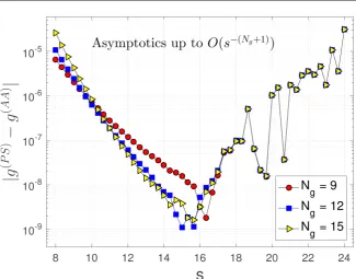
= , the observed value of parameter η in experiments. We will explore other values of η in subsequent sections.

In Figure 1, we plot the difference between _g( )PS

( )

_{s and g}( )AA

_{( )}

_{s as a} function of s for several different values of Ng. Three asymptotic approximations respectively with Ng =9, Ng =12 and Ng =15 are tested. For all 3 values of

Ng, especially for Ng =12 and Ng =15, Figure 1 demonstrates clearly the ex-istence of an overlapping valid region for the two numerical formulas. For s val-ues smaller than 17, there is a visible discrepancy among the three curves because in this region _g( )PS

( )

_{s −g}( )AA

( )

_{s is primarily attributed to the approximation} error in _g( )AA

( )

_{s which depends heavily on N}

g when s is not very large. For s values bigger than 17, the three curves almost coincide with each other due to the dominant effect of round-off errors in _g( )PS

( )

_{s which is independent of}

Ng. The overlapping region is in a neighborhood around [5] [6]. The asymptotic approximation with Ng =12 has the best performance since it reaches the

lowest minimum difference and attains the minimum difference at a smaller value of s, indicating that it is already valid even when s is not very large. In our subsequent simulations, we shall select Ng using this strategy. For Ng =12,

[image:10.595.212.538.57.312.2]

DOI: 10.4236/am.2018.96046 681 Applied Mathematics Figure 1. Difference between the power series summation _g( )PS

( )

_{s and the asymptotic} expansion _g( )AA

( )

_{s for various values of Ng.}

Numerical procedure:

• For s s≤ sw, g s

( )

is computed using the partial sum of the first Kf terms in power series summation (12).

( )

( )

(

)

(

)

( )1 1

0

1

, for 1

f k

K

k

sw k

g s s s s

k η η

+ −

= −

≈ ≤

Γ +

∑

(30)

on these numerical findings we adopt the numerical procedure below for where

Kf is the number of terms needed to make the truncation error well below the machine precision of IEEE double precision. In computations, we make the truncation error smaller than 10−20_{. Theoretically, K}

f has an a priori estimate ex-pressed in terms of s when s is moderately large. In practice, Kf is determined automatically in the numerical summation process by monitoring the magnitude of terms.

• For s s≥ sw, g s

( )

is calculated using the partial sum of terms up to

( )

(

Ng 1

)

O s− + in the asymptotic approximation (28).

( )

( ) (

)

( 1)

1 1 , for

g

k k

sw k

k N

g s f k s η s s

η

η − +

= ≤

≈

∑

− − ≥ ₍₃₁₎

The choice of ssw=15 and Ng =12 above is based on numerical minimi-zation of _g( )PS

( )

_{s −g}( )AA

( )

_{s with respect to}

(

_,

)

g

s N in the case of 0.1494

η

= . This particular set of

(

s Nsw, g

)

is for computing function g s

( )

at 0.1494

η

= . In a similar fashion, at each different value of η, an individual set of

(

s Nsw, g

)

is determined for that η and then used in evaluating g s

( )

.

ve-DOI: 10.4236/am.2018.96046 682 Applied Mathematics

rify properties (13) and (14) numerically, and thus demonstrate the well-posedness of the distribution density.

5. Numerical Verification of Well-Posedness

We first verify that g s

( )

defined by power series (12) is positive for all values of

s

>

0

at any parameter value of

η

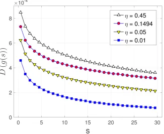
>0. To examine both the sign and the magnitude of g s

( )

, we use mapping D z

( )

, defined below, to display g s

( )

as D g s

(

( )

)

. Let

( )

1

0

0

sinh z

D z z

z

−  

≡ _{ }

 . (32)

where z0>0 is a design parameter depending on the range we like to focus on.

The mapping D z

( )

has several design features for showing the sign and for accommodating a huge range over many orders of magnitude.

• D z

( )

is an odd function of z, clearly showing the sign of z.

• D z

( )

is a monotonically increasing function of z, preserving any trend of

z.

• When z is significantly below z0, the mapping D z

( )

displays z in a

li-near scale:

( )

for 0

D z ≈z z z .

• When z is significantly above z0, the mapping D z

( )

displays z in a

lo-garithmic scale:

( )

0 0

0

2

ln z for

D z z z z

z

  ≈ _{ }

   .

We calculate g s

( )

vs s numerically for several representative values of 0

η

> , and plots D g s

(

( )

)

in Figure 2 with 4 0 10

z ₌ − _{. Function g s}

( )

_is pos-itive for all values of η we examined.

Next we verify that

_∫

₀+∞g s s

( )

d =1 for parameter

η

>0. We integrate the power series (12) to write out the cumulative distribution function (CDF), which becomes

( )

( )

₍

₍

( )

₎

₎

( )1

0 ₀

1 d

1 1

k

s _k

k

G s g u u s

k

η η

+

=

−

≡ =

Γ + +

∑

∫

. (33)

Again, theoretically power series (33) converges for all s, making G s

( )

a well defined function for all s. But in numerical computations with IEEE double precision, at large s, power series summation (33) suffers catastrophically from complete loss of accuracy. As a result, using the power series summation to compute G s

( )

at large s is not viable for demonstrating lims→+∞G s

( )

=1. In-stead, we consider the complementary cumulative distribution function at large

s, defined as

( )C

_{( )}

_{( )}

_d s

[image:12.595.212.539.74.341.2]

DOI: 10.4236/am.2018.96046 683 Applied Mathematics Figure 2. Plots of D g s

(

( )

)

for several values of parameter η. The mapping D z

( )

defined in (32) is designed for showing the sign and for accommodating a wide range of quantity z. The plots demonstrate that function g z

( )

is positive for all values of parameter η tested.

To verify

_∫

₀+∞g s s

( )

d =1_{, we only need to demonstrate numerically that}

( )

( )C

_{( )}

₁

G s G+ s = _{at some value of s. This allows us to select a value of s such}

that both G s

( )

and _G( )C

( )

_{s can be computed accurately.}

For s s≤ sw, G s

( )

can be accurately calculated using a partial sum of power series (33)

( )

₍

₍

( )

₎

₎

( )1

0

1

, for 1 1

f k

K

k

sw k

G s s s s

k

η η

+

= −

≈ ≤

Γ + +

∑

. (35)

For s s≥ sw, g s

( )

is well approximated by asymptotics (28). Using a partial sum of (28) with terms up to _{O s}

(

−(Ng+1)

)

_{to replace g s}

( )

_{in the integral of}

( )C

_{( )}

G s , we write out an asymptotic approximation for _G( )C

( )

_s

( )

_{( )}

_{( ) (}

₎

1 1 1 , for

g k

C k

sw k

k N

G s f k s η s s

η

η −

= ≤

≈ −

∑

− − + ≥ _{. (36)}

Results (35) and (36) suggest that quantity ₀+∞_{g u u G s G}

( )

d

( )

( )C

( )

_s

= +

∫

has

the optimal numerical accuracy if we evaluate it at s s= sw. Thus, we compute quantity

( )

( )C

( )

1

sw sw

G s +G s − _{and use it to judge if}

( )

0 g u ud 1

+∞

=

∫

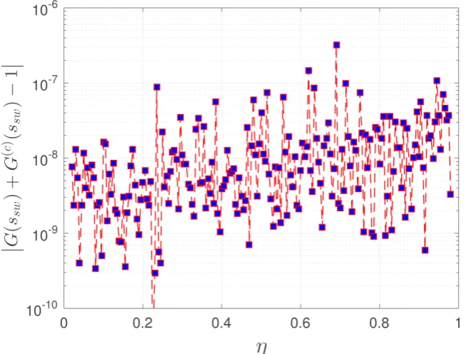
is satisfied.

Figure 3 plots

( )

( )C

( )

1

sw sw

G s +G s − _{vs parameter η. It is clear that for any} parameter value η in

( )

0,1 , the assertion

_∫

₀+∞g u u

( )

d =1 _{is indeed valid within}

[image:13.595.212.539.73.321.2]

DOI: 10.4236/am.2018.96046 684 Applied Mathematics Figure 3. The difference between

_∫

₀∞g u u

( )

d and 1 for different values of η.

In summary, we have numerically verified 1) g s

( )

>0 for s>0 and 2)

( )

0 g s sd 1

+∞

=

∫

. It follows that function g s

( )

defined by power series (12) is mathematically a proper distribution density.

With the property G

( )

+∞ =1 established, we write out a unified numerical procedure for computing function G s

( )

over the full range of s∈

(

0,+∞

)

,

( )

( )

(

(

)

)

( )

( ) (

)

1 =0

=0

1 1 1 for

1 1 for

f

g

K

k k

sw k

k _k

sw k

k N

f k s s s

G s

f k s s s

η

η

η

η

η

+

−

≤ 

− + + ≤

  ≈ 

− − + ≥

 

∑

∑

(37)

For readers’ convenience, we also summarize below the unified numerical procedure for computing function g s

( )

over the full range of s∈

(

0,+∞

)

_,

( )

( )

(

(

)

)

( )

( ) (

)

( )

1 1 0

1 1

1 1 for

1 for

f

g

K

k k

sw k

k k

sw k

k N

f k s s s

g s

f k s s s

η

η

η

η

η

+ −

=

− +

= ≤ 

− + ≤

  ≈ 

− − ≥

 

∑

∑

(38)

6. Pade Approximations

In the previous section, we verified G

( )

+∞ =1_{. We now impose this property as} a constraint at s= +∞ and construct a Pade approximation [7] [8] for G s

( )

based on its power series around s=0_{. As we will see, the Pade approximation}

provides an accurate and efficient approximation over the full range of

(

0,

)

DOI: 10.4236/am.2018.96046 685 Applied Mathematics

The power series of G s

( )

, given in (33), consists of integer powers of sη_. Accordingly, we use integer powers of sη _{in constructing the Pade} approxima-tion. For mathematical convenience, we write power series (33) in terms of

x s₌ η_{, in an abstract form}

( )

( )

₍

1

₎

1 1 , , 1 k k k k k

G s c x x s c

k η

η

+ +∞ = − = = = Γ +

∑

. (39)

Note that one can set c0=0 and start the summation at k=0 in (39).

Taking these features of function G s

( )

into consideration, we adopt a Pade approximation of order

[ ]

n n , of the form

( )

1 2 2 1 1

2 1

0 1 2 1

; n n n ,

n n

n

a x a x a x x

R s n x s

b b x b x b x x

η − − − − + + + + = = + + + + + 

 . (40)

where a0=0 follows from c0=0, and an=bn=1 follows from G

( )

+∞ =1 and normalization. There are

(

2 1n−

)

_{unknown coefficients in Pade} approxi-mation (40). To determine these coefficients, we multiply both (40) and (39) by

0

n k

k k=b x

∑

, and then match the _xk _{terms for 1≤ ≤k}

(

_{2 1n−}

)

_{. The product of} two power series has the expression:

0 0 0 0

k

k k k

k k j k j

k=b x k=c x k= j=b c− x

 

  _{ = }



  



∑



∑



∑ ∑

  .

For k in the range of n k≤ ≤

(

2 1n−

)

_{, equating the corresponding coefficients} of _xk _{terms on the left-hand side and on the right-hand sides yields equations} for the unknowns

{ }

bk .

(

)

1

0 , , 1, , 2 1

n

j k j k

j b c w k n n n

− − =

= = + −

∑

 (41)

where wk is known and has the expression

(

)

(

)

1,

, 1 2 1

k

k n k n

w _{c n k n}

−

= 

= _{− + ≤ ≤ −}

 (42)

Equation (41) is an

n n

×

linear system for

{

b b0, , ,1 bn−1

}

. Coefficients

{ }

bk are determined by solving linear system (41). Once coefficients

{ }

bk are known, we write out coefficients

{ }

ak by matching the coefficients of xk terms for 1≤ ≤k

(

n−1

)

.

(

)

1

0 , 1,2, , 1

k k j k j

j

a −b c− k n

=

=

∑

=  − (43)

To estimate the error of Pade approximation R s n

( )

; defined in (40), we use

( )

G s computed with the unified numerical procedure (37) as the “exact” solu-tion to compare with. We calculate the difference between the numerical value of

( )

G s and the Pade approximation R s n

( )

; . Figure 4 shows G s

( )

−R s n

( )

;

[image:15.595.213.538.58.308.2]

DOI: 10.4236/am.2018.96046 686 Applied Mathematics Figure 4. Discrepancy between G s

( )

and Pade approximation R s n

( )

; .

the asymptotic approximation in the overlapping region around s=15_{. The}

numerical error of procedure (37) varies with the magnitude of s. The numerical error is the largest in the overlapping region: below the overlapping region, the power series summation is less polluted by the round-off errors and thus is more accurate; above the overlapping region, the asymptotic approximation becomes more accurate. The numerical accuracy of G s

( )

calculated using (37) is signif-icantly higher than 10−8 _{when s is outside the overlapping region. This property} of G s

( )

will help us decipher the error behavior in higher order Pade ap-proximations.

When n is increased to n=5_{, the difference} G s

( )

−R s n

( )

; _{is below 10}−10 outside the overlapping region, implying that the error of Pade approximation is also below 10−10 _{outside the overlapping region. The difference G s}

( )

_{−R s n}

( )

_; increases significantly in the overlapping region. However, it is highly unlikely that the approximation error of Pade approximation jumps significantly only in the overlapping region while remaining below 10−10 _{outside the overlapping} re-gion. The Pade approximation consists of one rational function for all values of

s; it does not involve any switching. It is much more likely that the approxima-tion error of Pade approximaapproxima-tion actually remains below 10−10 _{over the full range} of s; the significant increase in G s

( )

−R s n

( )

; is solely caused by the increased numerical error of G s

( )

in the overlapping region. If this is true, then for

5

n= _{, the Pade approximation is already more accurate than the unified}

over-DOI: 10.4236/am.2018.96046 687 Applied Mathematics

lapping region is much more pronounced than in the case of n=5. The pattern of increase strongly suggests that it is caused by the increased numerical error of

( )

G s near the overlapping region. Figure 4 indicates that the true numerical error in Pade approximation is very likely below 10−12 _{throughout the full range} of s, much more accurate than the unified numerical procedure (37) in IEEE double precision.

We carry out single precision computations to support the assertion we made above that in finite precision arithmetic, Pade approximations can be more ac-curate than the power series even though the power series is theoretically exact in infinite precision arithmetic. We use the double precision result of G s

( )

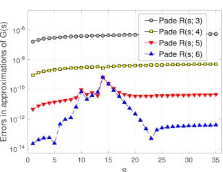
as the exact solution to compare with. We compute power series summation, asymptotics, and Pade approximations in single precision, and then examine the numerical errors in single precision results. Figure 5 shows the error behaviors of single precision results. As s increases, the power series summation starts los-ing accuracy due to the exponential growth of the largest term and the associated round-off error in summation. Meanwhile, as s increases, the approximation er-ror in asymptotics decreases and its numerical accuracy improves. In contrast, the numerical errors in Pade approximations remain fairly steady with respect to

[image:16.595.215.539.439.693.2]

s and decays very rapidly as n is increased. Pade approximation R s

( )

;3 is al-ready significantly more accurate than both the power series summation and the asymptotics in a large neighborhood of the overlapping region (for single preci-sion arithmetic, the overlapping region is around s=6_{). It is evident in Figure} 5 that the numerical error of R s

( )

;4 is primarily caused by round-off errors and its true approximation error is below the machine epsilon of single precision

DOI: 10.4236/am.2018.96046 688 Applied Mathematics

system. In single precision, the actually realized numerical accuracy of R s

( )

;4 is uniformly much higher than that of both the power series summation and the asymptotics over the full range of s.

Next, we construct a Pade approximation for density g s

( )

. Power series of

( )

g s around s=0 _{has the form}

( )

1

(

( )

)

1

0

d d

k k k G s x

g s s s c x

x

η η

η − − +∞

=

= =

∑



( )

(

)

(

1

)

,

1

k k

x s c

k η

η −

= =

Γ +

 . (44)

Note that since lim_x→+∞G s x

(

( )

)

=1, we have lim d

(

( )

)

0 d

x→+∞ _xG s x = in

(44), which suggests us to adopt a Pade approximation of order _

(

n−1

)

n_{, of}

the form

( )

1 0 1 1 1

1 0 1 1

; n n ,

n n

n

a a x a x

r s n s x s

b b x b x x

η− − − η

− −

 + + + 

=   =

+ + + +

 

   

  _  . (45)

There are 2n unknown coefficients in the Pade approximation of g s

( )

. To determine the coefficients, we multiply both (45) and (44) by

∑

k=₀

b x



k k, match the coefficients of _xk _{terms for 0≤ ≤k}

(

_{2 1n−}

)

_{to form a linear system, and} then solve for the unknowns, following a procedure similar to the one used in the Pade approximation of G s

( )

.

To assess the error of Pade approximation r s n

( )

; given in (45), we use

( )

g s computed with the unified numerical procedure (38) as the “exact” solu-tion to compare with. Figure 6 shows g s r s n

( ) ( )

− ; vs s for parameter value

0.1494

η

= _{. Four Pade approximations, respectively with, n = 3, 4, 5, and 6, are} shown where n is the highest power used in Pade approximation (45). The beha-viors of the Pade approximations for density g s

( )

are similar to those for the CDF g s

( )

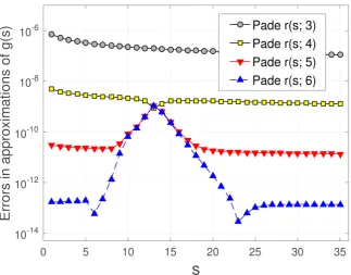
. In IEEE double precision, the actually realized numerical accuracy of the Pade approximations with n=5 _and n=6 _{is significantly better than}

that of numerical procedure (38). Again, in IEEE double precision, the smaller numerical error of the Pade approximations is mainly attributed to the fact that it contains only a few terms, and its numerical results are much less contami-nated with round-off errors.

7. Conclusion

[image:18.595.214.538.72.325.2]

DOI: 10.4236/am.2018.96046 689 Applied Mathematics Figure 6. Differences between density g s

( )

and its Pade approximations r s n

( )

; .

accuracy of 10−8 _{or better with IEEE double precision, over the full range of} ar-gument. Using this unified procedure, we verified numerically that for all para-meter values, the derived distribution density, i) is non-negative everywhere and ii) integrates to one. These results establish numerically that the derived distri-bution is indeed a proper density for all values of parameter, and thus, is well-posed. Furthermore, we developed efficient and accurate Pade approxima-tions for the distribution density and for the cumulative distribution function. In the computational environment of IEEE double precision, Pade approximations actually yield a much higher realized numerical accuracy than that of both the asymptotic approximation for large argument value and the power series for small argument value. The superior performance of Pade approximations is at-tributed to the fact that it attains high theoretical accuracy with only a few terms, which leads to less contamination with round-off errors and better realized nu-merical accuracy. In conclusion, we verified nunu-merically that the observed logis-tic dose-response relation can be explained solely based on a valid distribution of injury susceptibility. Rigorous proof of the well-posedness of the derived distri-bution density, however, still remains open.

8. Disclaimer

DOI: 10.4236/am.2018.96046 690 Applied Mathematics

References

[1] Glodsmith, M. (2015) Sound: A Very Short Introduction. Oxford University Press, Oxford.https://doi.org/10.1093/actrade/9780198708445.001.0001

[2] https://www.nidcd.nih.gov/health/noise-induced-hearing-loss

[3] Murphy, W.J., Khan, A. and Shaw, P.B. (2011) Analysis of Chinchilla Temporary and Permanent Threshold Shifts Following Impulsive Noise Exposure.

https://www.cdc.gov/niosh/surveyreports/pdfs/338-05c.pdf

[4] Chan, P., Ho, K. and Ryan, A.F. (2016) Impulse Noise Injury Model. Military Medi-cine, 181, 59-69.https://doi.org/10.7205/MILMED-D-15-00139

[5] Wang, H., Burgei, W.A. and Zhou, H. (2017) Interpreting Dose-Response Relation for Exposure to Multiple Sound Impulses in the Framework of Immunity. Health, 9, 1817-1842.https://doi.org/10.4236/health.2017.913132

[6] Wang, H., Burgei, W.A. and Zhou, H. (2018) Risk of Hearing Loss Caused by Mul-tiple Acoustic Impulses in the Framework of Biovariability. Health, 10, Article ID: 84786. https://doi.org/10.4236/health.2018.105048

[7] Bush, A.W. (1992) Perturbation Methods for Engineers and Scientists. CRC Press, Boca Raton.

[8] Hinch, E.J. (1991) Perturbation Methods. Cambridge University Press, New York.