Empirical safety stock estimation based on kernel and
GARCH models
Juan R. Traperoa,∗, Manuel Card´osb, Nikolaos Kourentzesc
aUniversidad de Castilla-La Mancha
Department of Business Administration, Ciudad Real 13071, Spain
bUniversidad Polit´ecnica de Valencia
Department of Business Administration, Valencia 46022, Spain
cLancaster University Management School
Department of Management Science, Lancaster, LA1 4Y X, UK
Abstract
Supply chain risk management has drawn the attention of practitioners and academics alike. One source of risk is demand uncertainty. Demand fore-casting and safety stock levels are employed to address this risk. Most pre-vious work has focused on point demand forecasting, given that the forecast errors satisfy the typical normal i.i.d. assumption. However, the real de-mand for products is difficult to forecast accurately, which means that—at minimum—the i.i.d. assumption should be questioned. This work analyzes the effects of possible deviations from the i.i.d. assumption and proposes empirical methods based on kernel density estimation (non-parametric) and GARCH(1,1) models (parametric), among others, for computing the safety stock levels. The results suggest that for shorter lead times, the normality deviation is more important, and kernel density estimation is most suitable. By contrast, for longer lead times, GARCH models are more appropriate because the autocorrelation of the variance of the forecast errors is the most important deviation. In fact, even when no autocorrelation is present in the original demand, such autocorrelation can be present as a consequence of the overlapping process used to compute the lead time forecasts and the uncertainties arising in the estimation of the parameters of the forecasting
∗Corresponding author.
model. Improvements are shown in terms of cycle service level, inventory investment and backorder volume. Simulations and real demand data from a manufacturer are used to illustrate our methodology.
Keywords: Forecasting, safety stock, risk, supply chain, prediction intervals, volatility, kernel density estimation, GARCH.
1. Introduction
Supply chain risk management (SCRM) is becoming an area of interest for researchers and practitioners, and the number of related publications is growing [1]. A critical review of SCRM was presented in [2]. An important source of risk is the uncertainty of future demand. When demand is un-usually large, a stockout may occur, with associated negative consequences. When demand is below expectations, the company is saddled with higher holding costs due to excess inventory. To mitigate such risks, companies use safety stocks, which are additional units beyond the stock required to meet a lead time forecasted demand. Different approaches can be utilized to calcu-late safety stock [3]. Although the most appropriate method depends on an organization’s circumstances, calculating the safety stock based on customer service is widely used, because it does not require knowledge of the stockout cost, which can be very difficult to estimate.
Demand uncertainty has been estimated by using both demand variabil-ity [4] and demand forecast error variability ([3], [5]). In this work, we follow the latter approach, given that future demand is unknown and must be fore-casted. Therefore, safety stocks are intended to prevent issues due to such demand forecast errors.
Demand forecast errors are typically assumed to be independent and iden-tically distributed (i.i.d.), following a Gaussian distribution with zero mean and constant variance. However, the forecast errors often do not satisfy these assumptions, which can cause the achieved service levels to deviate from the target levels, with increased inventory costs [6, 7, 8, 9]. Even when the dis-tribution assumptions are met, the uncertainties that arise when estimating the forecasting models are usually not considered [10, 11].
as promotional variables [14, 9, 15] or weather variables [9] via regression-type models; as well as considering temporal heteroscedastic processes [16, 17, 18, 9, 19]. Under the assumption that the improved forecasting model captures the underlying data process, a theoretical formula for the cumulative variance of the forecast error can be determined [20]. Then, the safety stock can be computed using that theoretical formula and assuming a statistical distribution.
Nonetheless, it would be unrealistic to assume that we could find the “true” demand model for each SKU, and even if such models did exist, it would not always be possible for companies to implement them in prac-tice. For instance, many companies judgmentally adjust statistical forecasts, which may induce forecast error biases [21, 22]. Furthermore, as pointed out by Fildes [23], companies often do not implement the latest research in fore-casting, relying instead on software vendors who have been shown to be very conservative. Moreover, the choice of demand forecasting model may not be under the control of the operations/inventory planning department [6].
For the aforementioned reasons, an alternative to the theoretical approach is an empirical, data-driven counterpart. In a univariate framework, the empirical approach involves collecting the observed lead time forecast errors of whatever forecasting model a company has available and, subsequently calculating the quantiles of interest to determine the safety stock. Note that in this empirical approach, we need to know neither the point forecasting model nor its parameters. This is potentially advantageous in the case of forecasting support systems, which often do not provide such information to users. For the case in which exogenous variables are available, Beutel and Minner [9], working within a multivariate framework, proposed a data-driven linear programming approach in which the inventory level could be optimized by minimizing a cost objective or subject to a service level constraint.
Several methodologies have been proposed to correct the problem that arises in a univariate framework in the case that the lead time forecast errors are biased. The authors of [6] adjusted the standard deviation of the forecast errors and reference [24] proposed a kernel-smoothing technique to cope with such unconditional bias. If the mean demand is autocorrelated and is not properly modeled, then the forecast error bias (if any) may be autocorrelated as well. Lee [8] developed a semi-parametric approach to estimate the critical fractiles for autocorrelated demand, where the conditional lead time demand forecast bias is a parametric linear function of the recent demand history and the quantile is obtained non-parametrically from the empirical distribution of the regression errors.
Likewise, the forecast errors for a given lead time may be heteroscedastic and deviate from normality [24, 8]. Non-normal residuals have been ad-dressed by means of kernel smoothing [24] and the empirical lead time error distribution quantile approach [8]. However, the case in which the lead time forecast errors exhibit conditional heteroscedasticity remains understudied.
In this work, the goal is to compute the safety stock for a given lead time using empirical methods based on the measured lead time forecast errors. Generalised AutoRegressive Conditional Heteroscedastic (GARCH) models [25] and exponential smoothing models [26] are investigated to overcome the assumption of the independence of the standard deviation of the lead time forecast errors and to exploit potential correlations.
To the best of the authors’ knowledge, this is the first time that GARCH models have been applied empirically to forecast lead time error standard deviations and compute safety stocks. Furthermore, we explore the use of empirical non-parametric approaches such as kernel density estimation [27], which is commonly utilized in prediction interval studies [28], although its use in supply chain applications has been less frequent [24, 29]. The pro-posed empirical approaches are also compared with the traditional supply chain theoretical approaches, which are based on i.i.d. assumptions, using both simulated data and real data from a manufacturing company. The performance of the different approaches are measured using inventory invest-ment, service level and backorder metrics. First, a newsvendor-type model is assumed, and subsequently, the results are compared with those of an order-up-to-level stock control policy.
proposed in this work. Section 5 explains the performance metrics used to assess the different methods. This section also provides implementation details for the alternative approaches. Simulation experiments are reported in Section6. A case study based on shipment data from a real manufacturer is presented in Section 7. Finally, Section 8presents concluding remarks.
2. Problem formulation
When the demand forecasting error is Gaussian i.i.d. with zero mean and constant variance, the safety stock (SS) for a target cycle service level (CSL), expressed as the target probability of no stockout during the lead time, can be computed as follows:
SS =kσL, (1)
wherek = Φ−1(CSL) is the safety factor, Φ(·) is the standard normal cumu-lative distribution function, and σL is the standard deviation of the forecast
errors for a certain lead time L, which is assumed to be constant and known. The main challenge associated with (1) is how to estimateσL. To do this,
we consider two approaches: a theoretical approach based on a forecasting model, in which an estimate of σ1 (one-step-ahead standard deviation of the
forecast error) is provided and an analytical expression that relates σL to
the forecasting model parameters, the lead time and σ1 is employed. The
estimation of σ1 is possible because the forecast updating step is usually
smaller than the lead time. Alternatively, an empirical parametric approach can also be employed in which σL is estimated directly from the lead time
forecast error. Here, the term parametric indicates that a known statistical distribution is assumed; normality is traditionally chosen for this purpose.
If the statistical distribution of the error is unknown, empirical non-parametric methods can be used instead. In that case, the safety stock calculation should be reformulated as follows:
SS =QL(CSL), (2)
where QL(CSL) is the forecast error quantile at the probability defined by
3. Theoretical approach
3.1. Estimation of σ1
Traditional textbooks suggest computingσ1 based on forecast error
met-rics. For instance, the mean squared error (MSE) is used in [3], and the mean absolute deviation (MAD) is used in [5]. However, the conversion fac-tor from the MAD toσ1 depends on the assumed statistical distribution, and
an inappropriate choice can result in a safety stock level that is inadequate to satisfy the required service level [3]. Therefore, hereafter, we use the MSE to estimate σ1, i.e. σ1 =
√
M SE . Moreover, the MSE estimation can be updated as new observations become available, as follows:
M SEt+1 =α0(yt−Ft)2+ (1−α0)M SEt, (3)
whereytis the actual value at timet,Ftis the forecast value for the same time
period, M SEt+1 is the MSE forecast for periodt+ 1 and α0 is a smoothing
constant that varies between 0 and 1. In this work,α0 and the initial value are optimized by minimizing the in-sample squared error following the suggestion by [30]. Note that (3) is the well-known single exponential smoothing (SES) method.
3.2. Estimation of σL
A theoretical formula forσL can be obtained given the following: σ1; the
forecast updating procedure; the value of the lead time (L), which is assumed to be constant and known; and the values of the smoothing constants used. According to [3], the exact relationship can be complicated. If we disregard the fact that the errors usually increase for longer forecast horizons and also assume that the forecast errors are independent over time [31], then
σL= √
Lσ1. (4)
It should be noted that expression (4) has been strongly criticized in [20] because there is no theoretical justification for its use and it can produce very inadequate results.
The authors of [32, 33, 34, 35] showed that when the demand can be modeled using a local level model (i.e., the model that underlies SES) with the parameter α, the conditional variance for the lead time demand is
σL=σ1
√ L
r
1 +α(L−1) + 1 6α
Interestingly, although (5) provides an exact relationship, the literature often relies on the approximation in (4) (see, for example, [6, 7]).
4. Empirical approach
The theoretical approach represented in (5) assumes that forecast errors are i.i.d., which means that we know the “true” model of the SKU’s demand. However, if there are doubts about the validity of the “true” model, then em-pirical approaches can be a useful alternative [20]. Given the complex nature of markets, clients, promotions, economic situation and so forth, assuming that we know the true demand model for each SKU would be unrealistic; consequently, empirical approaches must at least be tested.
Note that although empirical approaches have been shown to yield good results in other applications, such as the calculation of prediction intervals [20], they have rarely been used in SCRM [8].
4.1. Parametric approach
In these empirical parametric approaches, we retain the assumption that lead time forecast errors are normally distributed, but we relax the indepen-dent variance assumption by allowing σL to vary over time. An empirical
estimate of σL can be calculated as follows:
σL=
r Pn
t=1(et(L)−e¯(L))2
n , (6)
where et(L) = yL−FL = PLh=1yt+h−PLh=1Ft+h is the lead time forecast
error and ¯e(L) is the average error for the L under consideration.
4.1.1. Single exponential smoothing (SES)
Instead of using (6) to updateσLeach time a new observation is available,
we can use SES to directly update the cumulative MSE over the lead time [36, 26]. Likewise, we can update σL on the basis of the lead time forecast
error instead of the one-step-ahead forecasting error:
M SEL,t+1 =α00(yL−FL)2+ (1−α00)M SEL,t, (7)
wherepM SEL,t+1 is the forecast forσLat timet+ 1. Unlike in Eq. (3), the
FL is known as the overlapping temporal demand aggregation process [37],
which the authors recommend when a sufficient demand history is available (at least 24 observations). Similar to Eq. (3), both α00 and the initial value for Eq. (7) are optimized by minimizing the squared errors.
4.1.2. ARCH/GARCH models
Although exponential smoothing is the conventional approach in supply chain forecasting, when we are dealing with volatility forecasting other mod-els have been developed that may be good candidates for enhancing risk estimation and, therefore, safety stock determination.
In particular, the AutoRegressive Conditional Heteroscedasticity (ARCH) model introduced in [38] is one of the most important developments in risk modeling, and it may be well suited for our application. In ARCH models, the forecast error is expressed as t =σt·vt, where
σt2+1 =ω+
p X
i=1
ai2t−i+1, (8)
where ω is a constant, and ai are the respective coefficients of the p lags of vt that form an i.i.d. process. ARCH models express the conditional
vari-ance as a linear function of the p lagged squared error terms. Bollerslev in [25] proposed the generalized autoregressive conditional heteroscedasticity (GARCH) models that represent a more parsimonious and less restrictive ver-sion of the ARCH(p) models. GARCH(p,q) models express the conditional variance of the forecast error (or return) (t) at time t as a linear function of
both q lagged squared error terms and p lagged conditional variance terms. For example, a GARCH(1,1) model is given by:
σ2t+1 =ω+a12t +β1σt2. (9)
It should be noted that exponential smoothing has the same formulation as the integrated GARCH model (IGARCH) [39], withβ1 = 1−a1 andω = 0.
If we apply the GARCH(1,1) model to lead time forecasting error instead of to the one-step ahead forecasting error, Eq. (9) can be rewritten as follows:
σL,t2 +1 =ω0+a012L,t+β10σ2L,t. (10)
4.2. Non-parametric approach
Some demand distributions exhibit important asymmetries, particularly when they are subject to promotional periods or special events. In these cases, the typical normality assumption for forecasting errors does not hold. Non-parametric approaches, in which the safety stock is calculated in accor-dance with (2), are well suited for overcoming this problem. Here, we use two well-known non-parametric methods: (i) kernel density estimation and (ii) empirical percentile.
4.2.1. Kernel density estimation
This technique represents the probability density function f(x) of the lead time forecast errors without requiring assumptions concerning the data distribution. The kernel density formula for a series X at a point x is given by
f(x) = 1
N h N X
j=1
K
x−Xj h
, (11)
where N is the sample size,K(·) is the kernel smoothing function, which in-tegrates to one andhis the bandwidth [27]. In the cited reference (on p. 43), it is shown that the optimal kernel function, often called the Epanechnikov kernel, is:
Ke(t) =
( 3
4√5 1− 1 5t
2
−√5≤t ≤√5
0 otherwise (12)
Although the choice of h is still a topic of debate in the statistics literature, the following optimal bandwidth for a Gaussian kernel is typically chosen [27,28]:
hopt = 0.9AN−1/5, (13)
where A is an adaptive estimate of the spread given by
A=min(standard deviation,interquantile range/1.34) (14)
The CSL quantile, denoted byQL(CSL), can be estimated non-parametrically
4.2.2. Empirical percentile
The well known percentile indicates the value below which a given per-centage of observations fall. When calculating empirical percentiles the re-quested value is typically linearly interpolated from the available values.
5. Evaluation of the alternative approaches
5.1. Point forecasting
Before evaluating various approaches for measuring forecast error volatil-ity, we must first define the point forecasting function. The point forecasting algorithm yields a measure of the central tendency of the forecast density function. This value and the resulting forecast errors are used as the inputs to the variability forecasting methods described in Sections 3 and 4. Note that the same point forecast is used in all cases, regardless of the variability forecasting approach considered.
In this work, SES is used to produce point forecasts for two reasons. First, SES is widely used in business applications [40,41], and it is consistent with common practice, in which a company may not be using the optimal forecast-ing model due to either a lack of expertise or the availability of only a limited set of forecasting models in the software to which it has access. Second, we use SES as a benchmark because an analytical expression is available to com-pute the lead time forecasting error variance (see Eq. (5)), which requires an estimate of the value of α used in SES-based point forecasting. Such a forecasting method can be formulated as
Ft+h =αyt+ (1−α)Ft, (15)
where 0 ≤ α ≤ 1 and h is the forecasting horizon. Given the recursive nature of exponential smoothing, it is necessary to initialize the algorithm. We determine both the initial value and the α value by minimizing the in-sample mean squared error. Note that the lead time demand forecast is
FL=
PL
h=1Ft+h =L·Ft+1.
5.2. Inventory performance metrics
[43] transformed the inventory investment and backorder metrics into scale-independent measures that can easily summarize metrics across products by dividing them by the average in-sample demand, we follow the same approach here.
The way in which such inventory metrics are parameterized depends on the stock control policy. Here, we follow a newsvendor-type policy as in [9,8], where the critical fractile minimizes the expected cost by balancing the costs of understocking and overstocking [31]. We also study the critical fractile estimation problem with a fixed replenishment lead time, in which such a critical fractile solution is repeatedly applied for a multi-period inventory model [8]. The inventory metrics are the achieved CSL, which is estimated as the percentage of iterations where the lead time demand realizations fall below the estimated lead time demand quantile for determined target CSL values (critical fractiles). Backorders, by which we mean the amount of unsatisfied demand, are calculated in two steps. First, we calculate the sum of the demand realizations that exceed the estimated target CSL for each SKU, and second, we calculate the average of that sum across SKUs. Since we are interested in the safety stock, the average inventory investment is calculated as the average value of the so-called scaled safety stock, which is the safety stock divided by the in-sample average demand. All three metrics are calculated on the hold-out sample. In Section 6.4, the implementation of a periodic-review order-up-to-level stock control policy is also considered, and its results are compared with those of the newsvendor policy. Note that an order-up-to-level stock control policy is more appropriate when products are sold over a long time horizon with numerous replenishment opportunities and, thus, there is no need to dispose of excess inventory [45].
In this work, the target CSL values are set to 85%, 90%, 95% and 99% for both simulations and real data.
5.3. Implementation of the approaches
6. Simulation results
In this section, we describe four simulation experiments conducted to ex-plore the performance of the aforementioned empirical parametric and non-parametric approaches when there are deviations from the Gaussian i.i.d. assumptions. We study what happens when (i) the normality assumption does not hold for different sample sizes, (ii) the homoscedasticity and inde-pendent variance assumptions do not hold, and (iii) the lead time varies.
The simulations are assessed in terms of newsvendor inventory perfor-mance metrics (achieved CSL, scaled safety stock and backorders). To extend these simulation results to another well-known stock control policy, the last simulation study (iv) investigates the relationship between the newsvendor and order-up-to-level inventory performance metrics.
In these experiments, we divided the total sample into three parts. We used the first 20% of the data to estimate the parameters (initial value and smoothing parameter) for the point forecasting method and the next 50% to estimate the parameters for the volatility forecasting methods: SES, kernel density estimation, empirical percentile and GARCH(1,1). Note that em-pirical methods are estimated using data which have not been employed to produce the point forecasts, [46, 47, 48]. The remainder of the data was reserved as a hold-out sample for evaluation purposes.
6.1. Effects of sample size and demand distribution
To explore the influence of the demand distribution on the safety stock calculation, we employed three distributions: (i) normal, (ii) log-normal and (iii) gamma. Using this approach, we could observe any issues when the demand does not follow a normal distribution. Note that the log-normal distribution is reasonable when products are subject to promotional periods, during which the observed demand is higher than the baseline demand. The gamma distribution has previously been used in the literature [9, 29, 49] to assess violations of the normality assumption.
provide a mean of 150 and a skewness of 9.6, with the latter being used as a non-normality measure. The resulting parameter values for the log-normal distribution wereµ= 4.7 andσ= 0.7, while for the gamma distribution they were a= 0.04 (shape parameter) and b= 3,449 (scale parameter).
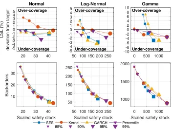
Figure 1 shows the trade-off curves for a sample size of 50 observations and a lead time of 1 period. The upper plots show the deviations from the target CSL in percentage vs. the scaled safety stock. For example, with a normal distribution and a target CSL of 85%, denoted by the smallest marker, the CSL deviation for SES is approximately -1% (i.e., undercoverage with an achieved CSL of 84%). The closer the lines are to zero deviation, the better the performance is considered to be. The lower panels plot the relationship between backorders and scaled safety stocks. Note that the different target CSLs are organized from the smallest-size marker (85%) to the largest-size marker (99%).
The left column of Figure 1 (both upper and lower panels) shows the trade-off curves for the normally distributed demand. As expected, SES and GARCH perform reasonably well and produce a slight systematic undercov-erage, whereas the kernel method produces a systematic overcoverage that is reduced for the highest target CSL. When the target is 99%, the empiri-cal percentile method achieves a remarkable lower CSL, which also implies a higher volume of backorders.
The middle column of Figure1presents the corresponding trade-off curves for the log-normal demand distribution. The non-parametric approaches (kernel and percentile) successfully achieve the highest and lowest target CSLs (99% and 85%, respectively), whereas the parametric approaches (SES and GARCH) do not. Therefore, when the forecast errors are skewed, the typical assumption of normality results in CSL values that deviates from their targets, and the non-parametric approaches seem more robust in this case.
20 30 40 -5 -4 -3 -2 -10 1 2 3 4 5 CSL (%)
deviation from target
Normal
Over-coverage
Under-coverage
SES Kernel GARCH Percentile 50 100 150 200 250
-5 -4 -3 -2 -1 0 1 2 3 4 5 Log-Normal Over-coverage Under-coverage
85% 90% 95% 99%
0 500 1000 -10 -8 -6 -4 -2 0 2 4 6 8 10 Gamma Over-coverage Under-coverage
85% 90% 95% 99%
20 30 40 Scaled safety stock 10
20 30
Backorders
50 100 150 200 250 Scaled safety stock 50
100 150 200 250
0 500 1000 Scaled safety stock 1000
[image:14.612.131.483.122.387.2]1500 2000
Figure 1: Trade-off curves for a sample size of 50 observations. Left column: normal distribution; middle column: log-normal distribution; right column: gamma distribution.
yield high backorder values for low CSL values and vice versa. By contrast, the parametric approaches yield backorder values that vary less strongly with the CSL value.
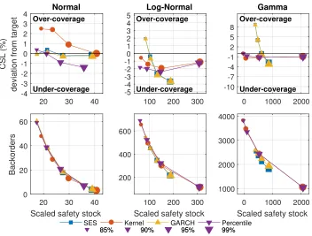
Figure 2 shows the corresponding trade-off curves when the sample size is increased to 100 observations. Again, the non-parametric approaches are better able to capture the asymmetry of the forecast errors at the highest and lowest CSLs (99% and 85%) for both the log-normal and gamma simu-lated demands. When the distribution is normal, all methods show similar performance in achieving values close to the target CSLs, although the kernel method results in systematically higher CSLs than expected.
The same conclusions are drawn when the sample size is further increased from 100 to 500 observations.
deterio-20 30 40 -4 -3 -2 -1 0 1 2 3 4 CSL (%)
deviation from target
Normal
Over-coverage
Under-coverage
SES Kernel GARCH Percentile
100 200 300 -5 -4 -3 -2 -1 0 1 2 3 4 5 Log-Normal Over-coverage Under-coverage
85% 90% 95% 99%
0 1000 2000 -10 -7 -4 -1 2 5 8 Gamma Over-coverage Under-coverage
85% 90% 95% 99%
20 30 40
Scaled safety stock
0 20 40 60
Backorders
100 200 300
Scaled safety stock
200 400 600
0 1000 2000
Scaled safety stock
[image:15.612.131.483.247.514.2]1000 2000 3000 4000
rates when the sample size is small since they are data-driven approaches. When the distribution is normal, the parametric approaches work well, as expected, although there is undercoverage when the sample size is small be-cause the parameters are not known and must be estimated [10]. The kernel method results in overcoverage, and the percentile method is more sensi-tive to small sample sizes. The overcoverage of the kernel method is due to the bandwidth selection, which establishes a compromise between bias and variance [27]. Because correlations of the forecast error variance are not considered in these simulations, the GARCH model does not exhibit any significant advantage over the SES model.
6.2. Demand with time-varying volatility
In this experiment, we performed two sets of simulations with time-varying volatility. In the first case, the demand followed a normal distri-bution with a constant mean (µ = 150) and two different standard devia-tions (σ1 = 25 and σ2 = 50); the sample size was 500 observations, and the
lead time was 1 period. σ1 was used for the time periods corresponding to
1:50, 101:226 and 351:425, with the purpose of ensuring the occurrence of volatility changes in both the in-sample periods and the hold-out sample. In the second case, the demand was simulated with a constant mean of 50 and a stochastic term that followed a GARCH(1,1) model, with the parameters
ω = 0.01, a1 = 0.4 and β1 = 0.5. In both cases, 100 simulations were run.
Figure 3 depicts the average trade-off curves obtained by each consid-ered technique for both experiments. The right column shows the trade-off curves for the first experiment with volatile abrupt changes. Regarding backorders, the SES and GARCH methods yield slightly lower backorders for similar scaled safety stocks. With respect to CSL deviations, the SES and GARCH methods provide overcoverage for lower targets and undercov-erage for the highest target. The kernel method produces overcovundercov-erage for each target, which is reduced for larger target CSLs, whereas the Percentile method achieves a CSL deviation close to zero.
are lower than those of their non-parametric counterparts, even for lower scaled safety stocks.
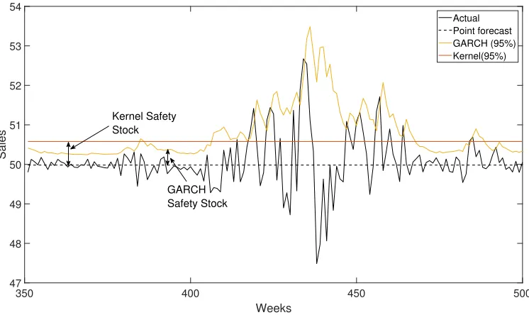
These results can be interpreted as follows: (i) When the forecast errors are subject to variance autocorrelation, GARCH models are a promising al-ternative for computing safety stocks that deserves further exploration. The best option that has been commonly applied thus far is SES [50,3], which can be seen as a particular case of GARCH models [39]. (ii) These results are also important because they suggest that the level of backorders can provide an indication of potential autocorrelation in the forecast error variance. In other words, when parametric approaches provide a level of backorders lower than non-parametric methods do, this may indicate a potential variance autocor-relation. To support this argument, Figure 4 shows the actual values and point forecasts for one Monte Carlo simulation on the hold-out sample for a CSL target of 95%. The same plot also depicts the safety stocks computed using the kernel and GARCH methods. We can see that the GARCH method is able to adapt to periods of high/low volatility, whereas the kernel method is not. Interestingly, although the kernel and GARCH methods result in similar numbers of stockouts during high-volatility periods and consequently produce similar achieved CSLs, the level of backorders is much higher when the kernel approach is used. Similarly, during periods of low volatility, the average safety stock yielded by the kernel method is greater than that of the GARCH method, and thus, the inventory investment is also higher with the kernel approach.
6.3. Influence of the lead time
In the simulations reported above, the lead time was set to 1 period. In this section, we investigate the influence of the lead time on the safety stock computation. For this experiment, we set the lead time to 4 periods, the sample size to 500 observations and each simulation was repeated 100 times. We used a demand process that followed an ARIMA(0,1,1) model with additional Gaussian innovations of zero mean and a standard deviation of σ = 2, where θ = −0.75. We used that ARIMA model because SES is optimal for such a model; thus, all differences among the evaluated methods are independent of the point forecasting model. The value of θ = −0.75 corresponds to a theoretical exponential smoothing constant of α = (1 +
0.5 1 1.5 2 -3
-2 -1 0 1 2 3
CSL (%)
deviation from target
Volatility simulated by GARCH(1,1) Over-coverage
Under-coverage
SES Kernel GARCH Percentile
0.5 1 1.5 2
Scaled safety stock
0 2 4
Backorders
20 40 60
-3 -2 -1 0 1 2
3 Volatility abrupt change Over-coverage
Under-coverage
85% 90% 95% 99%
20 40 60
Scaled safety stock
[image:18.612.132.480.240.538.2]0 200 400 600
350 400 450 500 Weeks
47 48 49 50 51 52 53 54
Sales
Actual Point forecast GARCH (95%) Kernel(95%)
Kernel Safety Stock
[image:19.612.119.492.124.346.2]GARCH Safety Stock
Figure 4: Example results from one Monte Carlo simulation
could also apply the theoretical approaches represented in Eqs. (4) and (5), hereafter denoted by σL(4) and σL(5), respectively. Recall that the SES,
kernel, GARCH and percentile methods are based on empirical lead time forecast errors.
Figure5shows that σL(4) produces a lower CSL and a higher number of
backorders thanσL(5) does because of the simplifications assumed in the case
ofσL(4); thus, our findings agree with those of [20] regarding the inadequacy
of σL(4). The percentile, kernel and GARCH methods, along with σL(5),
achieve CSLs very close to the targets, although the kernel method does so with a higher scaled safety stock. Interestingly, in terms of the CSL, SES per-forms worse than the non-parametric approaches, although GARCH perper-forms well. Regarding backorders, GARCH achieves very good performance—even better than that of σL(5). In the discussion of the time-varying simulations
8 10 12 14 16 18 20 22 24 26 28
-10-8
-6 -4
-20
2 4 6 8 10
CSL (%)
deviation from target
Over-coverage
Under-coverage
SES Kernel GARCH Percentile L(4) L(5)
8 10 12 14 16 18 20 22 24 26 28
Scaled safety stock 0
50 100 150
Backorders
[image:20.612.130.480.123.398.2]85% 90% 95% 99%
Figure 5: Trade-off curves for a demand that follows an ARIMA(0,1,1) model and a lead time of 4 periods
may originate from two sources: (i) The first possible source is overlapping temporal demand aggregation, as suggested by the fact that our results agree with those reported by [37], which indicate that the overlapping approach reduces inventory backorder volumes while maintaining the same volumes of held inventory. Note that such a variance autocorrelation due to overlapping may be present even when the original demand is independent; (ii) Similarly, the authors of [10] showed that when the parameters of the forecasting model are unknown and must be estimated, the forecast errors are correlated even when the demand is independent.
6.4. Stock control policies
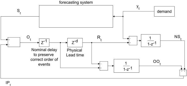
periodic-review, order-up-to stock control policy following the work of [51], as shown in Figure 6.
As in the previous experiment, the demand was described by a constant component (50 units) plus an ARIMA(0,1,1) component with θ = −0.75, a standard deviation of σ = 2 and a sample size of 500 observations. Each simulation was repeated 100 times. The ordering decision for an order-up-to-level policy is expressed as follows:
Ot=St−IPt, (16)
where Ot, St and IPt denote the ordering decision, order-up-to level and
inventory position, respectively, at timet. Note that the review interval is 1. The inventory position can be defined in terms of the net stock (N St) and
outstanding orders (OOt):
IPt=N St+OOt, (17)
where N St is
N St=
1
1−z−1(Rt−yt), (18)
where Z−1 is a Z-transform such as Z−1yt = yt−1 and Rt represents the
received orders. We use the variableN Stto compute the typical stock control
metrics. In other words, the achieved CSL is calculated as the proportion of the time periods in which N St is greater than zero given that a new
replenishment order is sent every time period, meaning that the cycle is unity. Backorders are calculated by summing the negative values of N St
across time and subsequently averaging across SKUs. Finally, the inventory investment is estimated as the average of the positiveN Stvalues across time
periods and SKUs.
The order-up-to level is updated every period:
St =FL+kσL, (19)
whereFLis the lead time forecast over Lperiods. Thus, in every period, the
retailer updates the order-up-to level with the current estimates of FL and σL. Note that St requires the estimation of the safety stock kσL.
The main difference between the block diagram model presented in [51] and the one shown in Figure 6 lies in σL. In [51], σL is not computed, and
Figure 6: Order-up-to-level stock control policy plus a forecasting system based on Eq. (5)
increasing the lead time by one period). In our work, we focus on different ways to compute σL and how those affect the safety stock performance. For
this simulation, we use Eq. (5) to computeσL, although any of the methods
presented could be used because we are analyzing the relations between the newsvendor and order-up-to stock control metrics. The described simulation is implemented in SIMULINK. Recall thatLalready includes a nominal one-period order delay (Z−1) because of the sequence of events [51]; therefore, we now have L = d+ 1, where Z−d is the physical lead time delay. To be coherent with the previous section, the lead time is set to L = 4; therefore
d = 3. The sequence of events is the following [51]: 1. receive, 2. satisfy demand, 3. count inventory, 4. place order.
86 88 90 92 94 96 98
Achieved CSL (Order up to)
86 88 90 92 94 96 98
Achieved CSL (Newsvendor)
5 10 15 20 25 30 35 40 45
Backorders (Order up to)
10 20 30 40
Backorders (Newsvendor)
1 2 3 4 5 6 7
Average net stock (Order up to)
12 14 16 18 20 22 24
Scaled safety stock (Newsvendor)
[image:23.612.111.499.124.373.2]85% 90% 95% 99%
Figure 7: Relationships between the newsvendor and order-up-to-level stock control policy metrics for target CSL values of 85%, 90%, 95% and 99%
by the scaled safety stock, is greater than the inventory investment of the order-up-to policy measured by the average net stock. Nevertheless, as in the case of the other metrics, the correlation between the scaled safety stock and the average net stock for different target CSLs is very high. Therefore, the simulation results reported in the previous sections for the newsvendor stock policy can be easily extrapolated to another well-known policy, namely, the order-up-to-level stock control policy.
7. Case study data
can be used to assess the robustness of the proposed methods to point fore-casts obtained using a method that does not perfectly match the unknown underlying data-generating process. This is a common situation both in re-search and in practice because identifying the true process is not trivial, as discussed before. To verify that SES is a reasonable method to provide point forecasts for this dataset, we compared the forecasting accuracy of the SES with that of ARIMA(p, d, q) models automatically identified by minimizing the Bayesian information criterion (BIC) [52] for p = (1,2,3), q = (1,2,3), and d = (0,1). For the point forecasting exercise, we designated 70% of the data as the hold-in sample and the rest as the hold-out sample. We normalized the sales for each SKU with respect to the corresponding mean in the hold-in sample to aggregate the results for all SKUS. The results are summarized in Table 1.
Table 1: Comparison of forecasting accuracy between SES and ARIMA models Error metric SES Automatic ARIMA
Mean(RMSE) 0.64 0.72
Median(RMSE) 0.60 0.65
In Table 1, Mean(RMSE) denotes the result of computing the root mean square error for each SKU on the hold-out sample and then averaging across all SKUs. By computing the median instead of the mean of the per-SKU RMSEs, we obtain the Median(RMSE) results reported in the second row. Overall, the SES method achieves a lower forecasting error than the auto-matic ARIMA models. This is not surprising since, as mentioned previously, the data do not exhibit any evident trends and/or seasonality.
Regarding the volatility forecasting exercise, as in the simulations, the data were split into three subsets. Again, SKU sales were normalized with respect to the hold-in sample means to aggregate the results for all SKUS in the trade-off curves.
the point forecasts. For the shortest lead time of 1 week, the null hypothesis of normality is rejected for 88.2% of the SKUs, and the null hypothesis of no conditional heteroscedasticity is rejected for 28.2%. Note the influence of the lead time on the statistical tests. As the lead time increases, the percentage of SKUs that do not pass the normality test decreases, as a consequence of the central limit theorem. By contrast, the percentage of SKUs that exhibit heteroscedasticity increases with the lead time. This may be due to the overlapping aggregation process and the estimation of the parameters, as explained in Section 6.3, where the influence of different lead times was analyzed.
Table 2: Percentages of the SKUs that do not pass the Jarque-Bera and Engle tests at the 5% significance level for different lead times
Lead time Jarque-Bera test (%) Engle test (%)
1 88.2 28.4
2 82.1 91.7
3 74.7 98.7
4 69.4 98.7
To test the adequacy of the GARCH(1,1) model on this real dataset, we computed the BIC for a general GARCH(p,q) model with p=1,2,3 and q=1,2,3 using the second part of the data devoted to optimizing the volatility models and a lead time of 4 weeks. The results show that GARCH(1,1) is a valid model because it minimizes the BIC for 97% of the SKUs.
Figures 8 and 9 show the trade-off curves of the manufacturer data for lead times of 1 and 4 weeks, respectively. In Figure8, because the lead time is 1 week, SES,σL(4) andσL(5) methods all produce the same results; thus, for
the sake of clarity, only the SES results are plotted. Because the conditional heteroscedasticity effect is lower for this lead time, the non-parametric kernel method produces lower deviations from the target for most CSLs (except 90%). For the highest target CSL (99%), the kernel method achieves the lowest CSL deviation and the lowest level of backorders, although at the expense of an increased scaled safety stock. This shows evidence of significant skewness in the data and is consistent with the results of the simulations, in which non-parametric approaches such as the kernel method produced better results for non-normal residuals.
50 100 150 200 250 -4
-2 0 2 4
CSL (%)
deviation from target
Over-coverage
Under-coverage
SES Kernel GARCH Percentile
50 100 150 200 250
Scaled safety stock
2 4 6
Backorders
[image:26.612.132.479.124.419.2]85% 90% 95% 99%
Figure 8: Trade-off curves for the manufacturer data for a lead time of 1 week
a lower CSL deviation and a lower level of backorders than σL(4) does, as
100 150 200 250 300 350 400 -10
-8 -6 -4 -2 0 2 4 6 8 10
CSL (%)
deviation from target
Over-coverage
Under-coverage
SES Kernel GARCH Percentile L(4) L(5)
100 150 200 250 300 350 400
Scaled safety stock
0 5 10 15 20
Backorders
[image:27.612.132.475.250.524.2]85% 90% 95% 99%
8. Conclusions
Despite the attention paid by both academics and practitioners to SCRM, the links between demand uncertainty and risks are still under-researched. One tool that supply chains typically employ to prevent further risks is safety stocks. This work examined empirical approaches, both parametric and non-parametric, for estimating the variability of the forecast errors and deter-mining the appropriate levels of safety stocks. In addition, these empirical methods were compared with the traditional theoretical methods described in the supply chain literature. Our intent was to provide recommendations for cases in which the assumption of normal i.i.d. forecast errors does not hold, which is common in practice.
The results of simulations show that empirical non-parametric approaches such as the kernel method are suitable when the statistical distribution of the forecast errors cannot be assumed to be normal. Additionally, if the vari-ance independence assumption cannot be guaranteed, empirical parametric approaches such as SES and GARCH offer a promising alternative. More-over, we found that when the GARCH or SES methods yields improved level of backorders, this improvement indicates the possibility of temporal het-eroscedasticity in the forecast errors. Under such circumstances, the GARCH method captures that heterocedasticity and achieves better performance in terms of the achieved CSL and backorder volume.
The results of the simulation experiments were evaluated for a newsven-dor stock policy, and the findings were compared with the outcomes obtained when the newsvendor policy was replaced with an order-up-to-level policy. The results showed high correlations between the inventory performance met-rics for the different stock control policies.
We also conducted experiments on real data and analyzed the influence of the lead time on the i.i.d. assumptions. For shorter lead times, the results were predominantly influenced by non-normality, and the kernel method pro-duced better results, particularly for higher target CSLs. As the lead time increased, conditional heteroscedasticity became dominant, which caused the empirical parametric methods (GARCH and SES) to produce better results. GARCH outperformed SES in terms of the achieved CSL, because SES is simply a particular case of the more general GARCH framework. These results on real data validate the conclusions obtained from the simulation exercises.
theoretical Eq. (4) is widely used because of its simplicity, if the forecasting model and parameters are known for a certain lead time, we recommend employing a more precise expression, such as Eq. (5), which is valid for the particular case of the SES forecasting model. Nevertheless, Eq. (5) does not consider the case in which the forecasting model parameters are not known and must be estimated, nor how the cumulative lead time demand forecasts are computed (using an overlapping or non-overlapping approach).
If sufficient data are available but the forecasting model and its param-eters cannot be determined (either because the forecasting support system does not provide such information, because the forecasts have been obtained using a combination of forecasting methods, or because there are doubts re-garding whether the forecast errors satisfy the i.i.d. assumptions), then we suggest the use of empirical approaches. For shorter lead times, the ker-nel method can effectively capture deviations from normality; for longer lead times, GARCH models are highly suitable and are a good alternative to SES, which has been traditionally utilized since the nineteen-sixties [50]. In this case, GARCH models can be a good choice even when the demand variance is uncorrelated.
Future research should address some of the limitations of this work. We analyzed SES and the GARCH(1,1) model for point and volatility forecasts, respectively. Future works should extend the applied GARCH models to incorporate exogenous variables that are available in advance, such as price discounts due to marketing campaigns. With regard to non-parametric meth-ods, the optimal selection of the kernel function and/or bandwidth also de-serves further investigation.
Acknowledgment
This work was supported by the European Regional Development Fund and the Spanish Government (MINECO/FEDER, UE) under project refer-ence DPI2015-64133-R. The authors would also like to thank the anonymous referees for their useful comments and suggestions.
References
[2] I. Heckmann, T. Comes, S. Nickel, A critical review on supply chain risk - definition, measure and modeling, Omega 52 (2015) 119 – 132.
[3] E. Silver, D. Pyke, D. Thomas, Inventory and Production Manage-ment in Supply Chains. Fourth Edition, CRC Press. Taylor and Francis Group, 2017.
[4] J. Heizer, B. Render, C. Munson, Operations Management: Sustainabil-ity and Supply Chain Management: Twelfth edition, Pearson Education, 2017.
[5] S. Nahmias, T. Olsen, Production and Operations Analysis: Seventh Edition, Waveland Press, 2015.
[6] M. P. Manary, S. P. Willems, Setting safety-stock targets at Intel in the presence of forecast bias, Interfaces 38 (2) (2008) 112–122.
[7] E. Porras, R. Dekker, An inventory control system for spare parts at a refinery: An empirical comparison of different re-order point methods, European Journal of Operational Research 184 (1) (2008) 101 – 132.
[8] Y. S. Lee, A semi-parametric approach for estimating critical fractiles under autocorrelated demand, European Journal of Operational Re-search 234 (1) (2014) 163 – 173.
[9] A. L. Beutel, S. Minner, Safety stock planning under causal demand fore-casting, International Journal of Production Economics 140 (2) (2012) 637 – 645.
[10] D. Prak, R. Teunter, A. Syntetos, On the calculation of safety stocks when demand is forecasted, European Journal of Operational Research 256 (2) (2017) 454 – 461.
[11] D. Prak, R. Teunter, A general method for addressing forecasting un-certainty in inventory models, International Journal of Forecasting. In press.
[13] T. L. Urban, Reorder level determination with serially-correlated de-mand, Journal of the Operational Research Society 51 (6) (2000) 762– 768.
[14] J. R. Trapero, N. Kourentzes, R. Fildes, Identification of sales forecast-ing models, J Oper Res Soc 66 (2) (2015) 299–307.
[15] N. Kourentzes, F. Petropoulos, Forecasting with multivariate temporal aggregation: The case of promotional modelling, International Journal of Production Economics 181, Part A (2016) 145 – 153.
[16] X. Zhang, Inventory control under temporal demand heteroscedasticity, European Journal of Operational Research 182 (1) (2007) 127 – 144.
[17] S. Datta, C. W. J. Granger, M. Barari, T. Gibbs, Management of supply chain: an alternative modelling technique for forecasting, Journal of the Operational Research Society 58 (11) (2007) 1459–1469.
[18] S. Datta, D. P. Graham, N. Sagar, P. Doody, R. Slone, O.-P. Hilmola, Forecasting and Risk Analysis in Supply Chain Management: GARCH Proof of Concept, Springer London, London, 2009, pp. 187–203.
[19] Y. Pan, R. Pavur, T. Pohlen, Revisiting the effects of forecasting method selection and information sharing under volatile demand in SCM appli-cations, IEEE Transactions on Engineering Management 63 (4) (2016) 377–389.
[20] C. Chatfield, Time-series forecasting, CRC Press, 2000.
[21] R. Fildes, P. Goodwin, M. Lawrence, K. Nikolopoulos, Effective forecast-ing and jugdmental adjustments: an empirical evaluation and strategies for improvement in supply-chain planning, International Journal of Fore-casting 25 (2009) 3–23.
[22] J. R. Trapero, D. J. Pedregal, R. Fildes, N. Kourentzes, Analysis of judgmental adjustments in the presence of promotions, International Journal of Forecasting 29 (2) (2013) 234 – 243.
[24] M. P. Manary, S. P. Willems, A. F. Shihata, Correcting heterogeneous and biased forecast error at Intel for supply chain optimization, Inter-faces 39 (5) (2009) 415–427.
[25] T. Bollerslev, Generalized autoregressive conditional heteroskedasticity, Journal of Econometrics 31 (3) (1986) 307 – 327.
[26] A. A. Syntetos, J. E. Boylan, Demand forecasting adjustments for service-level achievement, IMA Journal of Management Mathematics 19 (2) (2008) 175–192.
[27] B. Silverman, Density Estimation for Statistics and Data Analysis, Chapman & Hall/CRC Monographs on Statistics & Applied Probability, Taylor & Francis, Bristol, 1986.
[28] O. Isengildina-Massa, S. Irwin, D. L. Good, L. Massa, Empirical confi-dence intervals for USDA commodity price forecasts, Applied Economics 43 (26) (2011) 3789–3803.
[29] L. Strijbosch, R. Heuts, Modelling (s, Q) inventory systems: Parametric versus non-parametric approximations for the lead time demand distri-bution, European Journal of Operational Research 63 (1) (1992) 86 – 101.
[30] RiskMetrics, Riskmetrics technical document, Tech. rep., J.P. Mor-gan/Reuters (1996).
[31] S. Axs¨ater, Inventory Control: Third edition, International Series in Op-erations Research & Management Science, Springer International Pub-lishing, 2015.
[32] W. E. Wecker, The variance of cumulative demand forecasts, in: Grad-uate School of Business, Univ. of Chicago Waterloo, Canada Working Paper, 1979.
[33] F. R. Johnston, P. J. Harrison, The variance of lead-time demand, Jour-nal of the OperatioJour-nal Research Society 37 (3) (1986) 303–308.
[35] R. J. Hyndman, A. B. Koehler, J. K. Ord, R. D. Snyder, Forecasting with Exponential Smoothing: The State Space Approach, Springer-Verlag, Berlin, 2008.
[36] A. A. Syntetos, J. E. Boylan, On the stock control performance of inter-mittent demand estimators, International Journal of Production Eco-nomics 103 (1) (2006) 36 – 47.
[37] J. E. Boylan, M. Z. Babai, On the performance of overlapping and non-overlapping temporal demand aggregation approaches, International Journal of Production Economics 181 (2016) 136–144.
[38] R. F. Engle, Autoregressive conditional heteroscedasticity with esti-mates of the variance of united kingdom inflation, Econometrica: Jour-nal of the Econometric Society 50 (1982) 987–1007.
[39] D. B. Nelson, Stationarity and persistence in the GARCH(1,1) model, Econometric Theory 6 (3) (1990) 318–334.
[40] E. S. Gardner, Exponential smooothing: The state of the art, Journal of Forecasting 4 (1) (1985) 1–28.
[41] E. S. Gardner, Exponential smoothing: The state of the art, Part II, International Journal of Forecasting 22 (2006) 637–666.
[42] E. S. Gardner, Jr., Evaluating forecast performance in an inventory control system., Management Science 36 (4) (1990) 490 – 499.
[43] N. Kourentzes, On intermittent demand model optimisation and selec-tion, International Journal of Production Economics 156 (2014) 180 – 190.
[44] A. A. Syntetos, M. Z. Babai, E. S. Gardner, Forecasting intermittent in-ventory demands: simple parametric methods vs. bootstrapping, Jour-nal of Business Research 68 (8) (2015) 1746 – 1752.
[45] G. Cachon, C. Terwiesch, Matching supply with demand: an introduc-tion to operaintroduc-tions management: Third ediintroduc-tion, McGraw-Hill Educaintroduc-tion, 2013.
[47] L. Tashman, Out-of-sample tests of forecasting accuracy: an analysis and review, International Journal of Forecasting 16 (2000) 437–450.
[48] D. Barrow, N. Kourentzes, Distributions of forecasting errors of fore-cast combinations: implications for inventory management, Interna-tional Journal of Production Economics 177 (2016) 24–33.
[49] T. A. Burgin, The gamma distribution and inventory control, Journal of the Operational Research Society 26 (3) (1975) 507–525.
[50] R. Brown, Statistical forecasting for inventory control, New York: McGraw-Hill, 1959.
[51] J. Dejonckheere, S. M. Disney, M. R. Lambrecht, D. R. Towill, Mea-suring and avoiding the bullwhip effect: A control theoretic approach, European Journal of Operational Research 147 (2003) 567–590.