Posterior calibration and exploratory analysis for natural language
processing models
Khanh Nguyen
Department of Computer Science University of Maryland, College Park
College Park, MD 20742
Brendan O’Connor
College of Information and Computer Sciences University of Massachusetts, Amherst
Amherst, MA, 01003
Abstract
Many models in natural language process-ing define probabilistic distributions over linguistic structures. We argue that (1) the quality of a model’s posterior distribu-tion can and should be directly evaluated, as to whether probabilities correspond to empirical frequencies; and (2) NLP uncer-tainty can be projected not only to pipeline components, but also to exploratory data analysis, telling a user when to trust and not trust the NLP analysis. We present a method to analyze calibration, and apply it to compare the miscalibration of sev-eral commonly used models. We also con-tribute a coreference sampling algorithm that can create confidence intervals for a political event extraction task.1
1 Introduction
Natural language processing systems are imper-fect. Decades of research have yielded analyzers that mis-identify named entities, mis-attach syn-tactic relations, and mis-recognize noun phrase coreference anywhere from 10-40% of the time. But these systems are accurate enough so that their outputs can be used as soft, if noisy, indicators of language meaning for use in downstream analysis, such as systems that perform question answering, machine translation, event extraction, and narra-tive analysis (McCord et al., 2012; Gimpel and Smith, 2008; Miwa et al., 2010;Bamman et al., 2013).
To understand the performance of an ana-lyzer, researchers and practitioners typically mea-sure the accuracy of individual labels or edges among a single predicted output structurey, such as a most-probable tagging or entity clustering
arg maxyP(y|x)(conditional on text datax). 1See the extended version of this paper for software, ap-pendix, and acknowledgments sections:
http://brenocon.com/nlpcalib/ http://arxiv.org/abs/1508.05154
But a probabilistic model gives a probability distribution over many other output structures that have smaller predicted probabilities; a line of work has sought to control cascading pipeline errors by passing on multiple structures from earlier stages of analysis, by propagating prediction uncertainty through multiple samples (Finkel et al., 2006),
K-best lists (Venugopal et al., 2008; Toutanova et al., 2008), or explicitly diverse lists (Gimpel et al.,2013); often the goal is to marginalize over structures to calculate and minimize an expected loss function, as in minimum Bayes risk decod-ing (Goodman,1996;Kumar and Byrne,2004), or to perform joint inference between early and later stages of NLP analysis (e.g. Singh et al., 2013; Durrett and Klein,2014).
These approaches should work better when the posterior probabilities of the predicted linguistic structures reflect actual probabilities of the struc-tures or aspects of the strucstruc-tures. For example, say a model is overconfident: it places too much prob-ability mass in the top prediction, and not enough in the rest. Then there will be little benefit to us-ing the lower probability structures, since in the training or inference objectives they will be incor-rectly outweighed by the top prediction (or in a sampling approach, they will be systematically un-dersampled and thus have too-low frequencies). If we only evaluate models based on their top pre-dictions or on downstream tasks, it is difficult to diagnose this issue.
Instead, we propose to directly evaluate the cal-ibration of a model’s posterior prediction distri-bution. A perfectly calibrated model knows how often it’s right or wrong; when it predicts an event with 80% confidence, the event empirically turns out to be true 80% of the time. While perfect accuracy for NLP models remains an unsolved challenge, perfect calibration is a more achievable goal, since a model that has imperfect accuracy could, in principle, be perfectly calibrated. In this paper, we develop a method to empirically analyze calibration that is appropriate for NLP models (§3)
and use it to analyze common generative and dis-criminative models for tagging and classification (§4).
Furthermore, if a model’s probabilities are meaningful, that would justify using its proba-bility distributions for any downstream purpose, including exploratory analysis on unlabeled data. In§6 we introduce a representative corpus explo-ration problem, identifying temporal event trends in international politics, with a method that is de-pendent on coreference resolution. We develop a coreference sampling algorithm (§5.2) which projects uncertainty into the event extraction, in-ducing a posterior distribution over event frequen-cies. Sometimes the event trends have very high posterior variance (large confidence intervals),2 reflecting when the NLP system genuinely does not know the correct semantic extraction. This highlights an important use of a calibrated model: being able to tell a user when the model’s predic-tions are likely to be incorrect, or at least, not giv-ing a user a false sense of certainty from an erro-neous NLP analysis.
2 Definition of calibration
Consider a binary probabilistic prediction prob-lem, which consists of binary labels and proba-bilistic predictions for them. Each instance has a
ground-truth labely ∈ {0,1}, which is used for evaluation. The prediction problem is to gener-ate a predicted probability orprediction strength q ∈[0,1]. Typically, we use some form of a prob-abilistic model to accomplish this task, where q
represents the model’s posterior probability3of the instance having a positive label (y= 1).
Let S = {(q1, y1),(q2, y2),· · · (qN, yN)} be
the set of prediction-label pairs produced by the model. Many metrics assess the overall quality of how well the predicted probabilities match the data, such as the familiar cross entropy (negative average log-likelihood),
L`(~y, ~q) = N1
X
i
yilogq1
i + (1−yi) log
1 1−qi
or mean squared error, also known as the Brier scorewhenyis binary (Brier,1950),
L2(~y, ~q) = N1 X
i
(yi−qi)2
2We use the termsconfidence intervalandcredible
inter-valinterchangeably in this work; the latter term is debatably more correct, though less widely familiar.
3Whetherqcomes from a Bayesian posterior or not is ir-relevant to the analysis in this section. All that matters is that predictions are numbersq∈[0,1].
Both tend to attain better (lower) values whenqis near 1 wheny = 1, and near 0 wheny = 0; and they achieve a perfect value of 0 when allqi=yi.4
Let P(y, q) be the joint empirical distribution over labels and predictions. Under this notation,
L2 =Eq,y[y−q]2. Consider the factorization
P(y, q) =P(y |q)P(q)
where P(y | q) denotes the label empirical fre-quency, conditional on a prediction strength ( Mur-phy and Winkler, 1987).5 Applying this factor-ization to the Brier score leads to the calibration-refinement decomposition (DeGroot and Fienberg, 1983), in terms of expectations with respect to the prediction strength distributionP(q):
L2 = E|q[q{z−pq]2}
Calibration MSE
+ E|q[pq(1{z−pq)]}
Refinement
(1)
where we denotepq≡P(y= 1|q)for brevity.
Here, calibration measures to what extent a model’s probabilistic predictions match their cor-responding empirical frequencies. Perfect calibra-tion is achieved when P(y = 1 | q) = q for all
q; intuitively, if you aggregate all instances where a model predictedq, they should havey = 1atq
percent of the time. We define the magnitude of miscalibration using root mean squared error:
Definition 1(RMS calibration error).
CalibErr=qEq[q−P(y= 1|q)]2
The second term of Eq 1 refers to refinement, which reflects to what extent the model is able to separate different labels (in terms of the con-ditional Gini entropy pq(1−pq)). If the
predic-tion strengths tend to cluster around 0 or 1, the re-finement score tends to be lower. The calibration-refinement breakdown offers a useful perspective on the accuracy of a model posterior. This paper focuses on calibration.
There are several other ways to break down squared error, log-likelihood, and other probabilis-tic scoring rules.6 We use the Brier-based calibra-tion error in this work, since unlike cross-entropy
4These two loss functions are instances ofproper scoring
rules(Gneiting and Raftery,2007;Br¨ocker,2009).
5We alternatively refer to this aslabel frequencyor
empir-ical frequency. ThePprobabilities can be thought of as fre-quencies from the hypothetical population the data and pre-dictions are drawn from. Pprobabilities are, definitionally speaking, completely separate from a probabilistic model that might be used to generateqpredictions.
Algorithm 1 Estimate calibration error using adaptive binning.
Input: A set of N prediction-label pairs
{(q1, y1),(q2, y2),· · ·,(qN, yN)}.
Output:Calibration error. Parameter:Target bin sizeβ.
Step 1: Sort pairs by prediction valuesqkin ascending order. Step 2: For each, assign bin labelbk=j
k−1
β k
+ 1. Step 3: Define each binBias the set of indices of pairs that have the same bin label. If the last bin has size less than β, merge it with the second-to-last bin (if one exists). Let
{B1, B2,· · ·, BT}be the set of bins.
Step 4: Calculate empirical and predicted probabilities per bin:
ˆ pi= 1
|Bi|
X
k∈Bi
yk and qiˆ = 1
|Bi|
X
k∈Bi qk
Step 5: Calculate the calibration error as the root mean squared error per bin, weighted by bin size in case they are not uniformly sized:
CalibErr= v u u
t1
N T X
i=1
|Bi|(ˆqi−piˆ)2
it does not tend toward infinity when near prob-ability 0; we hypothesize this could be an issue since bothpandqare subject to estimation error.
3 Empirical calibration analysis
From a test set of labeled data, we can analyze model calibration both in terms of the calibration error, as well as visualizing thecalibration curve
of label frequency versus predicted strength. How-ever, computing the label frequenciesP(y = 1|q)
requires an infinite amount of data. Thus approx-imation methods are required to perform calibra-tion analysis.
3.1 Adaptive binning procedure
Previous studies that assess calibration in super-vised machine learning models (Niculescu-Mizil and Caruana, 2005; Bennett, 2000) calculate la-bel frequencies by dividing the prediction space into deciles or other evenly spaced bins—e.g.q∈ [0,0.1), q ∈ [0.1,0.2), etc.—and then calculat-ing the empirical label frequency in each bin. This procedure may be thought of as using a form of nonparametric regression (specifically, a regres-sogram; Tukey 1961) to estimate the function
f(q) = P(y = 1 | q)from observed data points. But models in natural language processing give very skewed distributions of confidence scores q
(many are near 0 or 1), so this procedure performs poorly, having much more variable estimates near
Algorithm 2 Estimate calibration error’s confi-dence interval by sampling.
Input: A set of N prediction-label pairs
{(q1, y1),(q2, y2),· · ·,(qN, yN)}.
Output:Calibration error with a 95% confidence interval. Parameter:Number of samples,S.
Step 1: Calculate {pˆ1,pˆ2,· · ·,pTˆ } from step 4 of
Algo-rithm 1.
Step 2: DrawSsamples. For eachs= 1..S,
• For each bini= 1..T, drawpˆ(s)
i ∼ N pi,ˆ σˆ2i, where ˆ
σ2
i = ˆpi(1−piˆ)/|Bi|. If necessary clip to [0,1]: ˆ
p(s)
i := min(1,max(0,pˆ(is)))
• Calculate the sample’sCalibErrfrom using the pairs (ˆqi,pˆ(s)
i )as per Step 5 of Algorithm 1.
Step 3: Calculate the 95% confidence interval for the calibra-tion error as:
CalibErravg±1.96 ˆserror
whereCalibErravg andserrorˆ are the mean and the stan-dard deviation, respectively, of the CalibErrs calculated from the samples.
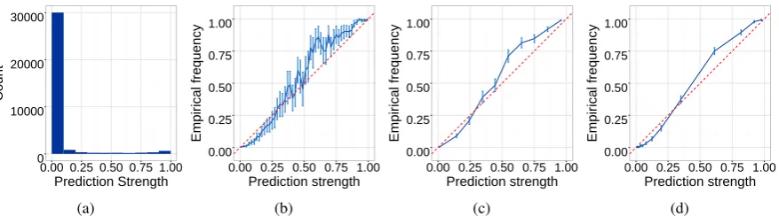
the middle of theqdistribution (Figure 1).
We propose adaptive binning as an alterna-tive. Instead of dividing the interval [0,1] into fixed-width bins, adaptive binning defines the bins such that there are an equal number of points in each, after which the same averaging proce-dure is used. This method naturally gives wider bins to area with fewer data points (areas that re-quire more smoothing), and ensures that these ar-eas have roughly similar standard errors as those near the boundaries, since for a bin withβ num-ber of points and empirical frequencyp, the stan-dard error is estimated bypp(1−p)/β, which is bounded above by0.5/√β. Algorithm 1 describes the procedure for estimating calibration error us-ing adaptive binnus-ing, which can be applied to any probabilistic model that predicts posterior proba-bilities.
3.2 Confidence interval estimation
calibra-0 10000 20000 30000
0.00 0.25 0.50 0.75 1.00
Prediction Strength
Count
(a)
0.00 0.25 0.50 0.75 1.00
0.00 0.25 0.50 0.75 1.00
Prediction strength
Empir
ical frequency
(b)
0.00 0.25 0.50 0.75 1.00
0.00 0.25 0.50 0.75 1.00
Prediction strength
Empir
ical frequency
(c)
0.00 0.25 0.50 0.75 1.00
0.00 0.25 0.50 0.75 1.00
Prediction strength
Empir
ical frequency
(d)
Figure 1: (a) A skewed distribution of predictions on whether a word has the NN tag (§4.2.2). Calibration curves produced by equally-spaced binning with bin width equal to 0.02 (b) and 0.1 (c) can have wide confidence intervals. Adaptive binning (with 1000 points in each bin) (d) gives small confidence intervals and also captures the prediction distribution. The confidence intervals are estimated as described in§3.1.
tion error estimate. Since we use bin sizes of at leastβ ≥200in our experiments, the central limit theorem justifies these approximations. We report all calibration errors along with their 95% confi-dence intervals calculated by Algorithm 2.7
3.3 Visualizing calibration
In order to better understand a model’s calibration properties, we plot the pairs
(ˆp1,q1ˆ),(ˆp2,q2ˆ),· · · ,(ˆpT,qˆT) obtained from
the adaptive binning procedure to visualize the
calibration curveof the model—this visualization is known as a calibration or reliability plot. It provides finer grained insight into the calibra-tion behavior in different prediccalibra-tion ranges. A perfectly calibrated curve would coincide with the y = x diagonal line. When the curve lies above the diagonal, the model is underconfident (q < pq); and when it is below the diagonal, the
model is overconfident (q > pq).
An advantage of plotting a curve estimated from fixed-size bins, instead of fixed-width bins, is that the distribution of the points hints at the refinement aspect of the model’s performance. If the points’ positions tend to cluster in the bottom-left and top-right corners, that implies the model is making more refined predictions.
4 Calibration for classification and tagging models
Using the method described in §3, we assess the quality of posterior predictions of several classi-fication and tagging models. In all of our
exper-7A major unsolved issue is how to fairly select the bin size. If it is too large, the curve is oversmoothed and tion looks better than it should be; if it is too small, calibra-tion looks worse than it should be. Bandwidth seleccalibra-tion and cross-validation techniques may better address this problem in future work. In the meantime, visualizations of calibration curves help inform the reader of the resolution of a particular analysis—if the bins are far apart, the data is sparse, and the specific details of the curve are not known in those regions.
iments, we set the target bin size in Algorithm 1 to be 5,000 and the number of samples in Algo-rithm 2 to be 10,000.
4.1 Naive Bayes and logistic regression 4.1.1 Introduction
Previous work on Naive Bayes has found its prob-abilities to have calibration issues, in part due to its incorrect conditional independence assump-tions (Niculescu-Mizil and Caruana, 2005; Ben-nett, 2000;Domingos and Pazzani, 1997). Since logistic regression has the same log-linear repre-sentational capacity (Ng and Jordan, 2002) but does not suffer from the independence assump-tions, we select it for comparison, hypothesizing it may have better calibration.
We analyze a binary classification task of Twit-ter sentiment analysis from emoticons. We col-lect a dataset consisting of tweets identified by the Twitter API as English, collected from 2014 to 2015, with the “emoticon trick” (Read,2005;Lin and Kolcz, 2012) to label tweets that contain at least one occurrence of the smiley emoticon “:)” as “happy” (y = 1) and others as y = 0. The smiley emoticons are deleted in positive examples. We sampled three sets of tweets (subsampled from the Decahose/Gardenhose stream of public tweets) with Jan-Apr 2014 for training, May-Dec 2014 for development, and Jan-Apr 2015 for testing. Each set contains 105 tweets, split between an equal
number of positive and negative instances. We use binary features based on unigrams extracted from the twokenize.py8 tokenization. We use the
scikit-learn(Pedregosa et al., 2011) implementa-tions of Bernoulli Naive Bayes and L2-regularized logistic regression. The models’ hyperparameters (Naive Bayes’ smoothing paramter and logistic re-gression’s regularization strength) are chosen to
8https://github.com/myleott/
[image:4.595.77.516.64.186.2]CalibErr=0.1048 ± 6.9E−03 0.00
0.25 0.50 0.75 1.00
0.00 0.25 0.50 0.75 1.00
Prediction strength
Empir
ical frequency
(a)
CalibErr=0.0409 ± 6.2E−03 0.00
0.25 0.50 0.75 1.00
0.00 0.25 0.50 0.75 1.00
Prediction strength
Empir
ical frequency
[image:5.595.309.522.64.187.2](b)
Figure 2: Calibration curve of (a) Naive Bayes and (b) lo-gistic regression on predicting whether a tweet is a “happy” tweet.
maximize the F-1 score on the development set.
4.1.2 Results
Naive Bayes attains a slightly higher F-1 score (NB 73.8% vs. LR 72.9%), but logistic regression has much lower calibration error: less than half as much RMSE (NB 0.105 vs. LR 0.041; Figure 2). Both models have a tendency to be undercon-fident in the lower prediction range and overconfi-dent in the higher range, but the tendency is more pronounced for Naive Bayes.
4.2 Hidden Markov models and conditional random fields
4.2.1 Introduction
Hidden Markov models (HMM) and linear chain conditional random fields (CRF) are another com-monly used pair of analogous generative and dis-criminative models. They both define a posterior over tag sequences P(y|x), which we apply to part-of-speech tagging.
We can analyze these models in the binary cal-ibration framework (§2-3) by looking at marginal distribution of binary-valued outcomes of parts of the predicted structures. Specifically, we examine calibration of predicted probabilities of individual tokens’ tags (§4.2.2), and of pairs of consecutive tags (§4.2.3). These quantities are calculated with the forward-backward algorithm.
To prepare a POS tagging dataset, we ex-tract Wall Street Journal articles from the En-glish CoNLL-2011 coreference shared task dataset from Ontonotes (Pradhan et al., 2011), using the CoNLL-2011 splits for training, development and testing. This results in 11,772 sentences for train-ing, 1,632 for development, and 1,382 for testtrain-ing, over a set of 47 possible tags.
We train an HMM with Dirichlet MAP us-ing one pseudocount for every transition and word emission. For the CRF, we use the L2
-regularized L-BFGS algorithm implemented in
CalibErr=0.0153 ± 5.1E−04 0.00
0.25 0.50 0.75 1.00
0.00 0.25 0.50 0.75 1.00
Prediction strength
Empir
ical frequency
(a)
CalibErr=0.0081 ± 3.5E−03 0.00
0.25 0.50 0.75 1.00
0.00 0.25 0.50 0.75 1.00
Prediction strength
Empir
ical frequency
[image:5.595.76.289.66.185.2](b)
Figure 3: Calibration curves of (a) HMM, and (b) CRF, on predictions over all POS tags.
CRFsuite(Okazaki,2007). We compare an HMM to a CRF that only uses basic transition (tag-tag) and emission (tag-word) features, so that it does not have an advantage due to more features. In order to compare models with similar task perfor-mance, we train the CRF with only 3000 sentences from the training set, which yields the same accu-racy as the HMM (about 88.7% on the test set). In each case, the model’s hyperparameters (the CRF’s L2 regularizer, the HMM’s pseudocount) are selected by maximizing accuracy on the devel-opment set.
4.2.2 Predicting single-word tags
In this experiment, we measure miscalibration of the two models on predicting tags of single words. First, for each tag type, we produce a set of 33,306 prediction-label pairs (for every token); we then concatenate them across the tags for calibration analysis. Figure 3 shows that the two models exhibit distinct calibration patterns. The HMM tends to be very underconfident whereas the CRF is overconfident, and the CRF has a lower (better) overall calibration error.
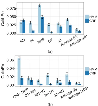
We also examine the calibration errors of the individual POS tags (Figure 4(a)). We find that CRF is significantly better calibrated than HMM in most but not all categories (39 out of 47). For example, they are about equally calibrated on pre-dicting the NN tag. The calibration gap between the two models also differs among the tags.
4.2.3 Predicting two-consecutive-word tags
0.000 0.025 0.050 0.075
NN IN NNP DT JJ
Average (5)Average (all)
Label
CalibErr
HMM CRF
(a)
0.00 0.02 0.04 0.06
NNP−NNPDT−NNNN−ININ−DTJJ−NNAverage (5)Average (100)
Label
CalibErr
HMM CRF
[image:6.595.74.281.63.285.2](b)
Figure 4: Calibration errors of HMM and CRF on predict-ing (a) spredict-ingle-word tags and (b) two-consecutive-word tags. Lower errors are better. The last two columns in each graph are the average calibration errors over the most common la-bels.
We report results for the top 5 and 100 most fre-quent tag pairs (Figure 4(b)). We observe a simi-lar pattern as seen from the experiment on single tags: the CRF is generally better calibrated than the HMM, but the HMM does achieve better cali-bration errors in 29 out of 100 categories.
These tagging experiments illustrate that, de-pending on the application, different models can exhibit different levels of calibration.
5 Coreference resolution
We examine a third model, a probabilistic model for within-document noun phrase coreference, which has an efficient sampling-based inference procedure. In this section we introduce it and ana-lyze its calibration, in preparation for the next sec-tion where we use it for exploratory data analysis.
5.1 Antecedent selection model
We use the Berkeley coreference resolution sys-tem (Durrett and Klein, 2013), which was origi-nally presented as a CRF; we give it an equivalent a series of independent logistic regressions (see appendix for details). The primary component of this model is a locally-normalized log-linear dis-tribution over clusterings of noun phrases, each cluster denoting an entity. The model takes a fixed input ofN mentions (noun phrases), indexed byi
in their positional order in the document. It posits that every mentionihas a latent antecedent selec-tion decision,ai ∈ {1, . . . , i−1,NEW}, denoting
which previous mention it attaches to, orNEWif it
is starting a new entity that has not yet been seen at a previous position in the text. Such a mention-mention attachment indicates coreference, while the final entity clustering includes more links im-plied through transitivity. The model’s generative process is:
Definition 2(Antencedent coreference model and sampling algorithm).
• Fori= 1..N, sample
ai∼ Z1iexp(wTf(i, ai, x))
• Calculate the entity clusters ase:=CC(a), the connected components of the antecedent graph having edges(i, ai)foriwhereai 6=
NEW.
Here x denotes all information in the document that is conditioned on for log-linear features f. e={e1, ...eM}denotes the entity clusters, where
each element is a set of mentions. There areM en-tity clusters corresponding to the number of con-nected components ina. The model defines a joint distribution over antecedent decisions P(a|x) =
Q
iP(ai|x); it also defines a joint distribution over
entity clusteringsP(e|x), where the probability of aneis the sum of the probabilities of allavectors that could give rise to it. In a manner similar to a distance-dependent Chinese restaurant process (Blei and Frazier,2011), it is non-parametric in the sense that the number of clustersM is not fixed in advance.
5.2 Sampling-based inference
For both calibration analysis and exploratory ap-plications, we need to analyze the posterior distri-bution over entity clusterings. This distridistri-bution is a complex mathematical object; an attractive ap-proach to analyze it is to draw samples from this distribution, then analyze the samples.
This antecedent-based model admits a very straightforward procedure to draw independent e samples, by stepping through Def. 2: indepen-dently sample eachaithen calculate the connected
components of the resulting antecedent graph. By construction, this procedure samples from the joint distribution ofe(even though we never com-pute the probability of any single clusteringe).
CalibErr=0.0087 ± 3.3E−03
0.00 0.25 0.50 0.75 1.00
0.00 0.25 0.50 0.75 1.00 Prediction strength
Empir
ical frequency
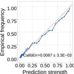
Figure 5: Coreference calibration curve for predicting whether two mentions belong to the same entity cluster.
compute—only slightly slower than calculating the MAP assignment (due to theexpand normal-ization for eachai). We implement this algorithm
by modifying the publicly available implementa-tion fromDurrett and Klein.9
5.3 Calibration analysis
We consider the following inference query: for a randomly chosen pair of mentions, are they coref-erent? Even if the model’s accuracy is compara-tively low, it may be the case that it is correctly calibrated—if it thinks there should be great vari-ability in entity clusterings, it may be uncertain whether a pair of mentions should belong together. Let`ijbe 1 if the mentionsiandjare predicted
to be coreferent, and 0 otherwise. Annotated data defines a gold-standard `(ijg) value for every pair
i, j. Any probability distribution overedefines a marginal Bernoulli distribution for every proposi-tion`ij, marginalizing oute:
P(`ij = 1|x) =
X
e
1{(i, j)∈e}P(e|x) (2)
where(i, j) ∈ eis true iff there is an entity ine that contains bothiandj.
In a traditional coreference evaluation of the best-prediction entity clustering, the model as-signs 1 or 0 to every`ij and the pairwise precision
and recall can be computed by comparing them to the corresponding`(ijg). Here, we instead compare theqij ≡ P(`ij = 1 | x,e) prediction strengths
against `(ijg) empirical frequencies to assess pair-wise calibration, with the same binary calibration analysis tools developed in§3 by aggregating pairs with similarqij values. Eachqij is computed by
averaging over 1,000 samples, simply taking the fraction of samples where the pair(i, j)is coref-erent.
9Berkeley Coreference Resolution System, version
1.1: http://nlp.cs.berkeley.edu/projects/
coref.shtml
We perform this analysis on the develop-ment section of the English CoNLL-2011 data (404 documents). Using the sampling inference method discussed in §5.2, we compute 4.3 mil-lions prediction-label pairs and measure their cali-bration error. Our result shows that the model pro-duces very well-calibrated predictions with less than 1% CalibErr (Figure 5), though slightly overconfident on middle to high-valued predic-tions. The calibration error indicates that it is the most calibrated model we examine within this pa-per. This result suggests we might be able to trust its level of uncertainty.
6 Uncertainty in Entity-based Exploratory Analysis
6.1 Entity-syntactic event aggregation
We demonstrate one important use of calibration analysis: to ensure the usefulness of propagating uncertainty from coreference resolution into a sys-tem for exploring unannotated text. Accuracy can-not be calculated since there are no labels; but if the system is calibrated, we postulate that un-certainty information can help users understand the underlying reliability of aggregated extractions and isolate predictions that are more likely to con-tain errors.
We illustrate with an event analysis application to count the number of “country attack events”: for a particular country of the world, how many news articles describe an entity affiliated with that country as the agent of an attack, and how does this number change over time? This is a simpli-fied version of a problem where such systems have been built and used for political science analysis (Schrodt et al., 1994;Schrodt,2012;Leetaru and Schrodt, 2013; Boschee et al., 2013; O’Connor et al., 2013). A coreference component can im-prove extraction coverage in cases such as “ Rus-sian troopswere sighted . . . andthey attacked. . . ” We use the coreference system examined in§5 for this analysis. To propagate coreference un-certainty, we re-run event extraction on multiple coreference samples generated from the algorithm described in§5.2, inducing a posterior distribution over the event counts. To isolate the effects of coreference, we use a very simple syntactic depen-dency system to identify affiliations and events. Assume the availability of dependency parses for a document d, a coreference resolution e, and a lexicon of country names, which contains a small set of wordsw(c)for each countryc; for example,
[image:7.595.107.253.53.198.2]f(c, e;xd)assesses whether an entityeis affiliated
with countrycand is described as the agent of an attack, based on document text and parses xd; f
returns true iff both:10
• There exists a mention i ∈ e described as country c: either its head word is in
w(c) (e.g. “Americans”), or its head word has an nmod or amod modifier in w(c)
(e.g. “American forces”, “president of the U.S.”); and there is only one unique country
camong the mentions in the entity.
• There exists a mention j ∈ ewhich is the
nsubjoragentargument to the verb “attack” (e.g. “they attacked”, “the forces attacked”, “attacked by them”).
For a givenc, we first calculate a binary variable for whether there is at least one entity fulfillingf
in a particular document,
a(d, c,ed) =
_
e∈ed
f(c, e;xd) (3)
and second, the number of such documents ind(t), the set ofNew York Timesarticles published in a given time periodt,
n(t, c,ed(t)) = X
d∈d(t)
a(d, c,ed) (4)
These quantities are both random variables, since they depend on e; thus we are interested in the posterior distribution ofn, marginalizing oute,
P(n(t, c,ed(t))|xd(t)) (5)
If our coreference model was highly certain (only one structure, or a small number of similar struc-tures, had most of the probability mass in the space of all possible structures), each document would have an a posterior near either 0 or 1, and their sum in Eq. 5 would have a narrow distribution. But if the model is uncertain, the distribution will be wider. Because of the transitive closure, the prob-ability of ais potentially more complex than the single antecedent linking probability between two mentions—the affiliation and attack information can propagate through a long coreference chain.
6.2 Results
We tag and parse a 193,403 article subset of the Annotated New York Times LDC corpus ( Sand-haus, 2008), which includes articles about world
10Syntactic relations are Universal Dependencies (de Marneffe et al., 2014); more details for the extrac-tion rules are in the appendix.
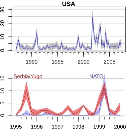
news from the years 1987 to 2007 (details in ap-pendix). For each article, we run the coreference system to predict 100 samples, and evaluatef on every entity in every sample.11 The quantity of interest is the number of articles mentioning at-tacks in a 3-month period (quarter), for a given country. Figure 6 illustrates the mean and 95% posterior credible intervals for each quarter. The posterior meanmis calculated as the mean of the samples, and the interval is the normal approxima-tionm±1.96s, wheresis the standard deviation among samples for that country and time period.
Uncertainty information helps us understand whether a difference between data points is real. In the plots of Figure 6, if we had used a 1-best coreference resolution, only a single line would be shown, with no assessment of uncertainty. This is problematic in cases when the model genuinely does not know the correct answer. For example, the 1993-1996 period of the USA plot (Figure 6, top) shows the posterior mean fluctuating from 1 to 5 documents; but when credible intervals are taken into consideration, we see that model does not know whether the differences are real, or were caused by coreference noise.
A similar case is highlighted at the bottom plot of Figure 6. Here we compare the event counts for Yugoslavia and NATO, which were engaged in a conflict in 1999. Did the New York Times de-vote more attention to the attacks by one particu-lar side? To a 1-best system, the answer would be yes. But the posterior intervals for the two coun-tries’ event counts in mid-1999 heavily overlap, indicating that the coreference system introduces too much uncertainty to obtain a conclusive an-swer for this question. Note that calibration of the coreference model is important for the credible in-tervals to be useful; for example, if the model was badly calibrated by being overconfident (too much probability over a small set of similar structures), these intervals would be too narrow, leading to in-correct interpretations of the event dynamics.
Visualizing this uncertainty gives richer infor-mation for a potential user of an NLP-based sys-tem, compared to simply drawing a line based on a single 1-best prediction. It preserves the gen-uine uncertainty due to ambiguities the system was unable to resolve. This highlights an alternative use ofFinkel et al.(2006)’s approach of sampling multiple NLP pipeline components, which in that work was used to perform joint inference. Instead
of focusing on improving an NLP pipeline, we can pass uncertainty on to exploratory purposes, and try to highlight to a user where the NLP system may be wrong, or where it can only imprecisely specify a quantity of interest.
Finally, calibration can help error analysis. For a calibrated model, the more uncertain a predic-tion is, the more likely it is to be erroneous. While coreference errors comprise only one part of event extraction errors (alongside issues in parse qual-ity, factivqual-ity, semantic roles, etc.), we can look at highly uncertain event predictions to understand the nature of coreference errors relative to our task. We manually analyzed documents with a 50% probability to contain an “attack”ing country-affiliated entity, and found difficult coreference cases.
In one article from late 1990, an “attack” event for IRQ is extracted from the sentence “But some political leaders said that they feared thatMr. Hus-sein might attack Saudi Arabia”. The mention “Mr. Hussein” is classified as IRQ only when it is coreferent with a previous mention “President Saddam Hussein of Iraq”; this occurs only 50% of the time, since in some posterior samples the coreference system split apart these two “Hussein” mentions. This particular document is addition-ally difficult, since it includes the names of more than 10 countries (e.g. United States, Saudi Ara-bia, Egypt), and some of the Hussein mentions are even clustered with presidents of other countries (such as “President Bush”), presumably because they share the “president” title. These types of er-rors are a major issue for a political analysis task; further analysis could assess their prevalence and how to address them in future work.
7 Conclusion
In this work, we argue that the calibration of pos-terior predictions is a desirable property of prob-abilistic NLP models, and that it can be directly evaluated. We also demonstrate a use case of having calibrated uncertainty: its propagation into downstream exploratory analysis.
Our posterior simulation approach for ex-ploratory and error analysis relates to posterior predictive checking (Gelman et al.,2013), which analyzes a posterior to test model assumptions; Mimno and Blei(2011) apply it to a topic model.
One avenue of future work is to investigate more effective nonparametric regression methods to better estimate and visualize calibration error, such as Gaussian processes or bootstrapped kernel
1990 1995 2000 2005
0
10
20
30
USA
0
10
20
30
1995 1996 1997 1998 1999 2000
0
5
10
[image:9.595.309.521.62.280.2]15 Serbia/Yugo. NATO
Figure 6: Number of documents with an “attack”ing country per 3-month period, and coreference posterior uncertainty for that quantity. The dark line is the posterior mean, and the shaded region is the 95% posterior credible interval. More examples in appendix.
density estimation.
Another important question is: what types of in-ferences are facilitated by correct calibration? In-tuitively, we think that overconfidence will lead to overly narrow confidence intervals; but in what sense are confidence intervals “good” when cal-ibration is perfect? Also, does calcal-ibration help joint inference in NLP pipelines? It may also assist calculations that rely on expectations, such as in-ference methods like minimum Bayes risk decod-ing, or learning methods like EM, since calibrated predictions imply that calculated expectations are statistically unbiased (though the implications of this fact may be subtle). Finally, it may be in-teresting to pursue recalibration methods, which readjust a non-calibrated model’s predictions to be calibrated; recalibration methods have been de-veloped for binary (Platt, 1999; Niculescu-Mizil and Caruana,2005) and multiclass (Zadrozny and Elkan, 2002) classification settings, but we are unaware of methods appropriate for the highly structured outputs typical in linguistic analysis. Another approach might be to directly constrain
CalibErr = 0during training, or try to reduce it as a training-time risk minimization or cost objec-tive (Smith and Eisner, 2006;Gimpel and Smith, 2010;Stoyanov et al., 2011;Br¨ummer and Dod-dington,2013).
References
David Bamman, Brendan O’Connor, and Noah A. Smith. Learning latent personas of film charac-ters. InProceedings of ACL, 2013.
Paul N. Bennett. Assessing the calibration of naive Bayes’ posterior estimates. Technical report, Carnegie Mellon University, 2000.
David M. Blei and Peter I. Frazier. Distance dependent Chinese restaurant processes. The Journal of Machine Learning Research, 12: 2461–2488, 2011.
Elizabeth Boschee, Premkumar Natarajan, and Ralph Weischedel. Automatic extraction of events from open source text for predictive forecasting. Handbook of Computational Ap-proaches to Counterterrorism, page 51, 2013. Glenn W. Brier. Verification of forecasts expressed
in terms of probability.Monthly weather review, 78(1):1–3, 1950.
Jochen Br¨ocker. Reliability, sufficiency, and the decomposition of proper scores. Quarterly Journal of the Royal Meteorological Society, 135(643):1512–1519, 2009.
Niko Br¨ummer and George Doddington. Likelihood-ratio calibration using prior-weighted proper scoring rules. arXiv preprint arXiv:1307.7981, 2013. Interspeech 2013. Marie-Catherine de Marneffe, Timothy Dozat,
Natalia Silveira, Katri Haverinen, Filip Gin-ter, Joakim Nivre, and Christopher D. Man-ning. Universal Stanford dependencies: A cross-linguistic typology. In Proceedings of LREC, 2014.
Morris H. DeGroot and Stephen E. Fienberg. The comparison and evaluation of forecasters. The statistician, pages 12–22, 1983.
Pedro Domingos and Michael Pazzani. On the op-timality of the simple Bayesian classifier under zero-one loss. Machine learning, 29(2-3):103– 130, 1997.
Greg Durrett and Dan Klein. Easy victories and uphill battles in coreference resolution. In
EMNLP, pages 1971–1982, 2013.
Greg Durrett and Dan Klein. A joint model for entity analysis: Coreference, typing, and link-ing. Transactions of the Association for Com-putational Linguistics, 2:477–490, 2014. Jenny Rose Finkel, Christopher D. Manning, and
Andrew Y. Ng. Solving the problem of cascad-ing errors: Approximate Bayesian inference for
linguistic annotation pipelines. InProceedings of the 2006 Conference on Empirical Methods in Natural Language Processing, pages 618– 626. Association for Computational Linguis-tics, 2006.
Andrew Gelman, John B. Carlin, Hal S. Stern, David B. Dunson, Aki Vehtari, and Donald B. Rubin. Bayesian data analysis. Chapman and Hall/CRC, 3rd edition, 2013.
Kevin Gimpel and Noah A. Smith. Rich source-side context for statistical machine translation. In Proceedings of the Third Workshop on Sta-tistical Machine Translation, pages 9–17, 2008. Kevin Gimpel and Noah A. Smith. Softmax-margin CRFs: Training log-linear models with cost functions. In Human Language Technolo-gies: The 2010 Annual Conference of the North American Chapter of the Association for Com-putational Linguistics, pages 733–736. Associ-ation for ComputAssoci-ational Linguistics, 2010. Kevin Gimpel, Dhruv Batra, Chris Dyer, and
Gre-gory Shakhnarovich. A systematic exploration of diversity in machine translation. In Pro-ceedings of the 2013 Conference on Empiri-cal Methods in Natural Language Processing, pages 1100–1111, Seattle, Washington, USA, October 2013. Association for Computational Linguistics. URL http://www.aclweb. org/anthology/D13-1111.
Tilmann Gneiting and Adrian E. Raftery. Strictly proper scoring rules, prediction, and estimation.
Journal of the American Statistical Association, 102(477):359–378, 2007.
Joshua Goodman. Parsing algorithms and met-rics. In Proceedings of the 34th Annual Meet-ing of the Association for Computational Lin-guistics, pages 177–183, Santa Cruz, Califor-nia, USA, June 1996. Association for Com-putational Linguistics. doi: 10.3115/981863. 981887. URLhttp://www.aclweb.org/ anthology/P96-1024.
Aria Haghighi and Dan Klein. Unsuper-vised coreference resolution in a nonparametric Bayesian model. InAnnual Meeting, Associa-tion for ComputaAssocia-tional Linguistics, volume 45, page 848, 2007.
Shankar Kumar and William Byrne. Minimum Bayes-risk decoding for statistical machine translation. In Daniel Marcu Susan Dumais and Salim Roukos, editors,HLT-NAACL 2004: Main Proceedings, pages 169–176, Boston, Massachusetts, USA, May 2 - May 7 2004. As-sociation for Computational Linguistics. Kalev Leetaru and Philip A. Schrodt. GDELT:
Global data on events, location, and tone, 1979– 2012. In ISA Annual Convention, volume 2, page 4, 2013.
Jimmy Lin and Alek Kolcz. Large-scale ma-chine learning at Twitter. InProceedings of the 2012 ACM SIGMOD International Conference on Management of Data, pages 793–804. ACM, 2012.
Michael C. McCord, J. William Murdock, and Branimir K. Boguraev. Deep parsing in Watson.
IBM Journal of Research and Development, 56 (3.4):3–1, 2012.
David Mimno and David Blei. Bayesian check-ing for topic models. In Proceedings of the 2011 Conference on Empirical Meth-ods in Natural Language Processing, pages 227–237, Edinburgh, Scotland, UK., July 2011. Association for Computational Linguis-tics. URL http://www.aclweb.org/ anthology/D11-1021.
Makoto Miwa, Sampo Pyysalo, Tadayoshi Hara, and Jun’ichi Tsujii. Evaluating dependency representations for event extraction. In Pro-ceedings of the 23rd International Confer-ence on Computational Linguistics (Coling 2010), pages 779–787, Beijing, China, Au-gust 2010. Coling 2010 Organizing Commit-tee. URL http://www.aclweb.org/ anthology/C10-1088.
Allan H. Murphy and Robert L. Winkler. A general framework for forecast verification.
Monthly Weather Review, 115(7):1330–1338, 1987.
Andrew Ng and Michael Jordan. On discrimina-tive vs. generadiscrimina-tive classifiers: A comparison of logistic regression and naive Bayes. Advances in neural information processing systems, 14: 841, 2002.
Alexandru Niculescu-Mizil and Rich Caruana. Predicting good probabilities with supervised learning. In Proceedings of the 22nd Interna-tional Conference on Machine Learning, pages 625–632, 2005.
Brendan O’Connor, Brandon Stewart, and Noah A. Smith. Learning to extract inter-national relations from political context. In
Proceedings of ACL, 2013.
Naoaki Okazaki. Crfsuite: a fast implemen-tation of conditional random fields (CRFs), 2007. URLhttp://www.chokkan.org/ software/crfsuite/.
F. Pedregosa, G. Varoquaux, A. Gramfort, V. Michel, B. Thirion, O. Grisel, M. Blondel, P. Prettenhofer, R. Weiss, V. Dubourg, J. Van-derplas, A. Passos, D. Cournapeau, M. Brucher, M. Perrot, and E. Duchesnay. Scikit-learn: Ma-chine learning in Python. Journal of Machine Learning Research, 12:2825–2830, 2011. John Platt. Probabilistic outputs for support vector
machines and comparisons to regularized like-lihood methods. In Advances in large margin classifiers. MIT Press (2000), 1999. URL
http://research.microsoft.com/ pubs/69187/svmprob.ps.gz.
Sameer Pradhan, Lance Ramshaw, Mitchell Mar-cus, Martha Palmer, Ralph Weischedel, and Ni-anwen Xue. CoNLL-2011 shared task: Mod-eling unrestricted coreference in Ontonotes. In Proceedings of the Fifteenth Conference on Computational Natural Language Learning: Shared Task, pages 1–27. Association for Com-putational Linguistics, 2011.
Jonathon Read. Using emoticons to reduce depen-dency in machine learning techniques for senti-ment classification. InProceedings of the ACL Student Research Workshop, pages 43–48. As-sociation for Computational Linguistics, 2005. Evan Sandhaus. The New York Times
Anno-tated Corpus. Linguistic Data Consortium, LDC2008T19, 2008.
Philip A. Schrodt. Precedents, progress, and prospects in political event data. International Interactions, 38(4):546–569, 2012.
Philip A. Schrodt, Shannon G. Davis, and Ju-dith L. Weddle. KEDS – a program for the machine coding of event data. Social Science Computer Review, 12(4):561 –587, December 1994. doi: 10.1177/089443939401200408. URL http://ssc.sagepub.com/ content/12/4/561.abstract.
InProceedings of the 2013 Workshop on Auto-mated Knowledge Base Construction, pages 1– 6. ACM, 2013.
David A. Smith and Jason Eisner. Minimum risk annealing for training log-linear models. In Pro-ceedings of the COLING/ACL 2006 Main Con-ference Poster Sessions, pages 787–794, Syd-ney, Australia, July 2006. Association for Com-putational Linguistics. URL http://www. aclweb.org/anthology/P06-2101. Veselin Stoyanov, Alexander Ropson, and Jason
Eisner. Empirical risk minimization of graphi-cal model parameters given approximate infer-ence, decoding, and model structure. In Interna-tional Conference on Artificial Intelligence and Statistics, pages 725–733, 2011.
Kristina Toutanova, Aria Haghighi, and Christo-pher D. Manning. A global joint model for se-mantic role labeling. Computational Linguis-tics, 34(2):161–191, 2008.
John W. Tukey. Curves as parameters, and touch estimation. InProceedings of the Fourth Berkeley Symposium on Mathematical Statis-tics and Probability, Volume 1: Contributions to the Theory of Statistics, pages 681–694, Berkeley, Calif., 1961. University of Califor-nia Press. URLhttp://projecteuclid. org/euclid.bsmsp/1200512189. Ashish Venugopal, Andreas Zollmann, Noah A.
Smith, and Stephan Vogel. Wider pipelines: N-best alignments and parses in MT training. In
Proceedings of AMTA, 2008.
Larry Wasserman. All of nonparametric statistics. Springer Science & Business Media, 2006. Bianca Zadrozny and Charles Elkan.