Improved Relation Extraction with Feature Rich Compositional Embedding Models

Improved Relation Extraction with

Feature-Rich Compositional Embedding Models

Matthew R. Gormley1⇤ _{and Mo Yu}2⇤_{and Mark Dredze}1 1_{Human Language Technology Center of Excellence}

Center for Language and Speech Processing Johns Hopkins University, Baltimore, MD, 21218

2_{Machine Intelligence and Translation Lab} Harbin Institute of Technology, Harbin, China

[email protected], {mrg, mdredze}@cs.jhu.edu

Abstract

Compositional embedding models build a representation (or embedding) for a linguistic structure based on its compo-nent word embeddings. We propose a Feature-rich Compositional Embedding Model (FCM) for relation extraction that

is expressive, generalizes to new domains, and is easy-to-implement. The key idea is to combine both (unlexicalized) hand-crafted features with learned word em-beddings. The model is able to directly tackle the difficulties met by traditional compositional embeddings models, such as handling arbitrary types of sentence an-notations and utilizing global information for composition. We test the proposed model on two relation extraction tasks, and demonstrate that our model outper-forms both previous compositional models and traditional feature rich models on the ACE 2005 relation extraction task, and the SemEval 2010 relation classification task. The combination of our model and a log-linear classifier with hand-crafted features gives state-of-the-art results. We made our implementation available for general use1_.

1 Introduction

Two common NLP feature types are lexical properties of words and unlexicalized linguis-tic/structural interactions between words. Prior work on relation extraction has extensively stud-ied how to design such features by combining dis-cretelexical properties (e.g. the identity of a word,

⇤⇤_{Gormley and Yu contributed equally.}

1_{https://github.com/mgormley/pacaya}

its lemma, its morphological features) with as-pects of a word’s linguistic context (e.g. whether it lies between two entities or on a dependency path between them). While these help learning, they make generalization to unseen words difficult. An alternative approach to capturing lexical informa-tion relies on continuous word embeddings2 _as

representative of words but generalizable to new words. Embedding features have improved many tasks, including NER, chunking, dependency pars-ing, semantic role labelpars-ing, and relation extrac-tion (Miller et al., 2004; Turian et al., 2010; Koo et al., 2008; Roth and Woodsend, 2014; Sun et al., 2011; Plank and Moschitti, 2013; Nguyen and Grishman, 2014). Embeddings can capture lexi-cal information, but alone they are insufficient: in state-of-the-art systems, they are used alongside features of the broader linguistic context.

In this paper, we introduce a compositional model that combines unlexicalized linguistic con-text and word embeddings for relation extraction, a task in which contextual feature construction plays a major role in generalizing to unseen data. Our model allows for the composition of embed-dings with arbitrary linguistic structure, as ex-pressed by hand crafted features. In the follow-ing sections, we begin with a precise construction of compositional embeddings using word embed-dings in conjunction with unlexicalized features. Various feature sets used in prior work (Turian et al., 2010; Nguyen and Grishman, 2014; Hermann et al., 2014; Roth and Woodsend, 2014) are

cap-2_{Such embeddings have a long history in NLP,} in-cluding term-document frequency matrices and their low-dimensional counterparts obtained by linear algebra tools (LSA, PCA, CCA, NNMF), Brown clusters, random projec-tions and vector space models. Recently, neural networks / deep learning have provided several popular methods for ob-taining such embeddings.

Class M1 M2 Sentence Snippet

(1) ART(M1,M2) a man a taxicab A mandrivingwhat appeared to be a taxicab

(2) PART-WHOLE(M1,M2) the southern suburbs Baghdad direction of the southern suburbsofBaghdad

[image:2.595.84.510.62.104.2]

(3) PHYSICAL(M2,M1) the united states 284 people in the united states , 284 peopledied

Table 1:Examples from ACE 2005. In (1) the word “driving” is a strong indicator of the relationART3_betweenM

1andM2.

A feature that depends on the embedding for this context word could generalize to other lexical indicators of the same relation (e.g. “operating”) that don’t appear withARTduring training. But lexical information alone is insufficient; relation extraction requires the identification of lexical roles: wherea word appears structurally in the sentence. In (2), the word “of” between “suburbs” and “Baghdad” suggests that the first entity is part of the second, yet the earlier occurrence after “direction” is of no significance to the relation. Even finer information can be expressed by a word’s role on the dependency path between entities. In (3) we can distinguish the word “died” from other irrelevant words that don’t appear between the entities.

tured as special cases of this construction. Adding these compositional embeddings directly to a stan-dard log-linear model yields a special case of our full model. We then treat the word embeddings as parameters giving rise to our powerful, efficient, and easy-to-implement log-bilinear model. The model capitalizes on arbitrary types of linguistic annotations by better utilizing features associated with substructures of those annotations, including global information. We choose features to pro-mote different properties and to distinguish differ-ent functions of the input words.

The full model involves three stages. First, it decomposes the annotated sentence into substruc-tures (i.e. a word and associated annotations). Second, it extracts features for each substructure (word), and combines them with the word’s em-bedding to form asubstructure embedding. Third, we sum over substructure embeddings to form a composed annotated sentence embedding, which is used by a final softmax layer to predict the out-put label (relation).

The result is a state-of-the-art relation extractor for unseen domains from ACE 2005 (Walker et al., 2006) and the relation classification dataset from SemEval-2010 Task 8 (Hendrickx et al., 2010).

Contributions This paper makes several contri-butions, including:

1. We introduce theFCM, a new compositional

embedding model for relation extraction. 2. We obtain the best reported results on

ACE-2005 for coarse-grained relation extraction in the cross-domain setting, by combiningFCM

with a log-linear model.

3. We obtain results on on SemEval-2010 Task 8 competitive with the best reported results. Note that other work has already been published that builds on the FCM, such as Hashimoto et al.

(2015), Nguyen and Grishman (2015), dos Santos

3_{In ACE 2005,ARTrefers to a relation between a person} and an artifact; such as a user, owner, inventor, or manufac-turer relationship

et al. (2015), Yu and Dredze (2015) and Yu et al. (2015). Additionally, we have extended FCM to

incorporate a low-rank embedding of the features (Yu et al., 2015), which focuses on fine-grained relation extraction for ACE and ERE. This paper obtains better results than the low-rank extension on ACE coarse-grained relation extraction.

2 Relation Extraction

In relation extraction we are given a sentence as in-put with the goal of identifying, for all pairs of en-tity mentions, what relation exists between them, if any. For each pair of entity mentions in a sen-tence S, we construct an instance (y,x), where

x = (M1, M2, S, A). S = {w1, w2, ..., wn} is

a sentence of length n that expresses a relation of type y between two entity mentions M1 and

M2, whereM1 andM2 are sequences of words in

S. Ais the associated annotations of sentenceS, such as part-of-speech tags, a dependency parse, and named entities. We consider directed rela-tions: for a relation type Rel, y=Rel(M1, M2) andy0_=Rel(M

2, M1) are different relations. Ta-ble 1 shows ACE 2005 relations, and has a strong label bias towards negative examples. We also consider the task of relation classification (Se-mEval), where the number of negative examples is artificially reduced.

as-sumed that the order of two entities in a relation are given while the relation type itself is unknown (Nguyen and Grishman, 2014; Nguyen and Grish-man, 2015). The standard relation extraction task, as adopted by ACE 2005 (Walker et al., 2006), uses long sentences containing multiple named en-tities with known types4_{and unknown relation}

di-rections. We are the first to apply neural language model embeddings to this task.

Motivation and Examples Whether a word is indicative of a relation depends on multiple prop-erties, which may relate to its context within the sentence. For example, whether the word is in-between the entities, on the dependency path be-tween them, or to their left or right may provide additional complementary information. Illustra-tive examples are given in Table 1 and provide the motivation for our model. In the next section, we will show how we develop informative repre-sentations capturing both the semantic information in word embeddings and the contextual informa-tion expressing a word’s role relative to the entity mentions. We are the first to incorporate all of this information at once. The closest work is that of Nguyen and Grishman (2014), who use a log-linear model for relation extraction with embed-dings as features for only the entity heads. Such embedding features are insensitive to the broader contextual information and, as we show, are not sufficient to elicit the word’s role in a relation.

3 A Feature-rich Compositional Embedding Model for Relations

We propose a general framework to construct an embedding of a sentence with annotations on its component words. While we focus on the rela-tion extracrela-tion task, the framework applies to any task that benefits from both embeddings and typi-cal hand-engineered lexitypi-cal features.

3.1 Combining Features with Embeddings

We begin by describing a precise method for con-structing substructure embeddings and annotated sentence embeddings from existing (usually un-lexicalized) features and embeddings. Note that these embeddings can be included directly in a log-linear model as features—doing so results in

4_{Since the focus of this paper is relation extraction, we} adopt the evaluation setting of prior work which uses gold named entities to better facilitate comparison.

a special case of our full model presented in the next subsection.

An annotated sentence is first decomposed into substructures. The type of substructures can vary by task; for relation extraction we consider one substructure per word5_{. For each substructure in}

the sentence we have a hand-crafted feature vec-tor fwi and a dense embedding vector ewi. We

represent each substructure as the outer product

⌦between these two vectors to produce a matrix, herein called asubstructure embedding: hwi =

fwi⌦ewi. The featuresfwi are based on the local

context inS and annotations inA, which can in-clude global information about the annotated sen-tence. These features allow the model to pro-mote different properties and to distinguish differ-ent functions of the words. Feature engineering can be task specific, as relevant annotations can change with regards to each task. In this work we utilize unlexicalized binary features common in relation extraction. Figure 1 depicts the con-struction of a sentence’s substructure embeddings. We further sum over the substructure embed-dings to form anannotated sentence embedding:

ex= n

X

i=1

fwi⌦ewi (1)

When both the hand-crafted features and word em-beddings are treated as inputs, as has previously been the case in relation extraction, this anno-tated sentence embedding can be used directly as the features of a log-linear model. In fact, we find that the feature sets used in prior work for many other NLP tasks are special cases of this simple construction (Turian et al., 2010; Nguyen and Grishman, 2014; Hermann et al., 2014; Roth and Woodsend, 2014). This highlights an im-portant connection: when the word embeddings are constant, our constructions of substructure and annotated sentence embeddings are just specific forms of polynomial (specifically quadratic) fea-ture combination—hence their commonality in the literature. Our experimental results suggest that such a construction is more powerful than directly including embeddings into the model.

3.2 The Log-Bilinear Model

Our full log-bilinear model first forms the sub-structure and annotated sentence embeddings from

054

055

056

057

058

059

060

061

062

063

064

065

066

067

068

069

070

071

072

073

074

075

076

077

078

079

080

081

082

083

084

085

086

087

088

089

090

091

092

093

094

095

096

097

098

099

100

101

102

103

104

105

106

107

Based on above ideas, we achieve a general model and can easily apply to model to an NLP task

without the need for designing model structures or selecting features from scratch. Specifically, if

we denote a instance as

(

y, S

)

, where

S

is an arbitrary language structure and

y

is the label for

the structure. Then we decompose the structure to some factors following

S

=

{

f

}

. For each

factor

f

, there is a list of

m

associated features

g

=

g

1

, g

2

, ..., g

m

, and a list of

t

associated words

w

f,

1

, w

f,

2

, ..., w

f,t

2

f

. Here we suppose that each factor has the same number of words, and there

is a transformation from the words in a factor to a hidden layer as follows:

h

f

=

e

w

f,1

:

e

w

f,2

:

...

:

e

w

f,t

·

W

,

(1)

where

e

w

i

is the word embedding for word

w

i

. Suppose the word embeddings have

d

e

dimensions

and the hidden layer has

d

h

dimensions. Here

W

= [

W

1

W

2

...

W

t

]

, each

W

j

is a

d

e

⇥

d

h

matrix,

is a transformation from the concatenation of word embeddings to the inputs of the hidden layer.

Then the sigmoid transformation will be used to get the values of hidden layer from its inputs.

Dev MRR

Test MRR

Model

Fine-tuning

supervison

1,000 10,000 100,000 1,000 10,000 100,000

SUM

_Y

-

_PPDB

-

46.95

_50.81

35.29

_36.81

30.69

_32.92

52.63

_57.23

_45.01

41.19

37.32

_41.23

RNN

(d=50)

Y

PPDB

45.67

30.86

27.05

54.84

39.25

35.49

RNN

(d=200)

Y

PPDB

48.97

33.50

31.13

53.59

40.50

38.57

FCT

N

PPDB

47.53

35.58

31.31

54.33

41.96

39.10

Y

PPDB

51.22

36.76

33.59

61.11

46.99

44.31

FCT

-

LM

49.43

37.46

32.22

53.56

42.63

39.44

Y

LM

+ PPDB 53.82

37.48

34.43

65.47

49.44

45.65

joint

LM

+ PPDB

56.53

41.41

36.45

68.52

51.65

46.53

Table 9: Performance on the semantic similarity task with PPDB data.

@`

@T

=

n

X

i

=1

@`

@R

⌦

f

w

i

⌦

e

w

i

,

(13)

@`

@e

w

=

n

X

i

=1

I

[

w

i

=

w

]

T

_@R

@`

f

w

i

(14)

T

:

n

X

i

=1

f

i

⌦

e

w

i

representation

(15)

T

n

X

i

=1

f

i

⌦

e

w

i

!

(16)

T

n

X

i

=1

f

i

⌦

e

w

i

!

=

n

X

i

=1

T

f

i

e

w

i

M

i

n

X

i

=1

f

i

⌦

e

w

i

(17)

(18)

+

(19)

(

w

i

, f

i

=

f

(

w

i

, S

))

(20)

w

i

2

S

(21)

T

(

⌦

f

w

i

⌦

e

w

i

)

,

(22)

(23)

2

,

0

0

(24)

2

,

1

,

2

,

2

,

2

,

3

0

(25)

054 055 056 057 058 059 060 061 062 063 064 065 066 067 068 069 070 071 072 073 074 075 076 077 078 079 080 081 082 083 084 085 086 087 088 089 090 091 092 093 094 095 096 097 098 099 100 101 102 103 104 105 106 107

Based on above ideas, we achieve a general model and can easily apply to model to an NLP task

without the need for designing model structures or selecting features from scratch. Specifically, if

we denote a instance as

(

y, S

)

, where

S

is an arbitrary language structure and

y

is the label for

the structure. Then we decompose the structure to some factors following

S

=

{

f

}

. For each

factor

f

, there is a list of

m

associated features

g

=

g

1

, g

2

, ..., g

m

, and a list of

t

associated words

w

f,1

, w

f,2

, ..., w

f,t

2

f

. Here we suppose that each factor has the same number of words, and there

is a transformation from the words in a factor to a hidden layer as follows:

h

f

=

e

wf,1

:

e

wf,2

:

...

:

e

wf,t

·

W

,

(1)

where

e

wi

is the word embedding for word

w

i

. Suppose the word embeddings have

d

e

dimensions

and the hidden layer has

d

h

dimensions. Here

W

= [

W

1

W

2

...

W

t

]

, each

W

j

is a

d

e

⇥

d

h

matrix,

is a transformation from the concatenation of word embeddings to the inputs of the hidden layer.

Then the sigmoid transformation will be used to get the values of hidden layer from its inputs.

Figure 1: Tensor representation of the FCT model. (a) Representation of an input sentence. (b)

Representation for the parameter space.

Based on above notations, we can represent each factor as the outer product between the feature

vector and the hidden layer of transformed embedding

g

f

⌦

h

f

. The we use a tensor

T

=

L

⌦

E

⌦

F

as in Figrure 1(b) to transform this input matrix to the labels. Here

L

is the set of labels,

E

refers to

all dimensions of hidden layer

(

|

E

|

= 200)

and

F

is the set of features.

In order to predict the conditional probability of a label

y

given the structure

S

, we have

P

(

y

|

S

;

T

) =

P

exp

{

s

(

y, S

;

T

)

}

y 2L

exp

{

s

(

y , S

;

T

)

}

,

(2)

where

s

(

y, S

;

T

)

is the score of label

y

computed with our model. Since we decompose the

struc-ture

S

to factors, each factor

f

i

2

S

will contribute to the score based on the model parameters.

Specifically, each label

y

corresponds to a slice of the tensor

T

y

, which is a matrix

(

y,

·

,

·

)

. Then

each factor

f

i

will contribute a score

s

(

y, f

i

) =

T

y

g

f

h

f

,

(3)

where correspond to tensor product, while in the case of Eq.(3), it has the equivalent form:

T

y

g

f

h

f

=

T

y

(

g

f

⌦

h

f

) = ( (

y,

·

,

·

)

·

g

f

)

T

h

f

.

In this way, the target score of label

y

given an instance

S

and parameter tensor

T

can be written as:

s

(

y, S

;

T

) =

n

X

i=1

s

(

y, f

i

;

T

) =

n

X

i=1

T

y

g

fi

h

fi

.

(4)

The

FCM

model only performs linear transformations on each view of the tensor, making the model

efficient and easy to implement.

Learning

In order to train the parameters we optimize the following cross-entropy objective:

`

(

D

;

T, W

) =

X

(y,S)2D

log

P

(

y

|

S

;

T, W

)

where

D

is the set of all training data.

We used AdaGrad [9] to optimize above

objective.

Therefore we are performing stochastic training;

and for each

in-stance

(

y, S

)

the loss function

`

=

`

(

y, S

;

T, W

)

=

log

P

(

y

|

S

;

T, W

)

.

Then

2

162

163

164

165

166

167

168

169

170

171

172

173

174

175

176

177

178

179

180

181

182

183

184

185

186

187

188

189

190

191

192

193

194

195

196

197

198

199

200

201

202

203

204

205

206

207

208

209

210

211

212

213

214

215

Classifier

Features

F1

SVM []

POS, prefixes, morphological, WordNet, dependency parse,

82.2

(Best in SemEval2010)

Levin classed, ProBank, FrameNet, NomLex-Plus,

Google n-gram, paraphrases, TextRunner

RNN

word embeddings, syntactic parse

_{word embeddings, syntactic parse, POS, NER, WordNet}

74.8

_77.6

MVRNN

word embeddings, syntactic parse

_{word embedding, syntactic parse, POS, NER, WordNet}

79.1

_82.4

FCM (fixed-embedding)

word embeddings, dependency parse, WordNet

82.0

FCM (fine-tuning)

word embeddings, dependency parse, WordNet

82.3

FCM + linear

word embeddings, dependency parse, WordNet

Table 2: Feature sets used in

FCM

.

References

[1] Yoshua Bengio, Holger Schwenk, Jean-S´ebastien Sen´ecal, Fr´ederic Morin, and Jean-Luc Gauvain. Neural

probabilistic language models. In

Innovations in Machine Learning

, pages 137–186. Springer, 2006.

[2] Ronan Collobert and Jason Weston. A unified architecture for natural language processing: Deep neural

networks with multitask learning. In

International conference on Machine learning

, pages 160–167.

ACM, 2008.

[3] Tomas Mikolov, Ilya Sutskever, Kai Chen, Greg Corrado, and Jeffrey Dean. Distributed representations

of words and phrases and their compositionality.

arXiv preprint arXiv:1310.4546

, 2013.

[4] Joseph Turian, Lev Ratinov, and Yoshua Bengio. Word representations: a simple and general method for

semi-supervised learning. In

Association for Computational Linguistics

, pages 384–394, 2010.

[5] Ronan Collobert. Deep learning for efficient discriminative parsing. In

International Conference on

Artificial Intelligence and Statistics

, 2011.

[6] Eric H Huang, Richard Socher, Christopher D Manning, and Andrew Y Ng. Improving word

represen-tations via global context and multiple word prototypes. In

Association for Computational Linguistics

,

pages 873–882, 2012.

[7] Richard Socher, Alex Perelygin, Jean Wu, Jason Chuang, Christopher D. Manning, Andrew Ng, and

Christopher Potts. Recursive deep models for semantic compositionality over a sentiment treebank. In

Empirical Methods in Natural Language Processing

, pages 1631–1642, 2013.

[8] Karl Moritz Hermann, Dipanjan Das, Jason Weston, and Kuzman Ganchev. Semantic frame identification

with distributed word representations. In

Proceedings of ACL

. Association for Computational Linguistics,

June 2014.

[9] John Duchi, Elad Hazan, and Yoram Singer. Adaptive subgradient methods for online learning and

stochastic optimization.

The Journal of Machine Learning Research

, 12:2121–2159, 2011.

[10] Iris Hendrickx, Su Nam Kim, Zornitsa Kozareva, Preslav Nakov, Diarmuid ´O S´eaghdha, Sebastian Pad´o,

Marco Pennacchiotti, Lorenza Romano, and Stan Szpakowicz. Semeval-2010 task 8: Multi-way

clas-sification of semantic relations between pairs of nominals. In

Proceedings of the SemEval-2 Workshop

,

Uppsala, Sweden, 2010.

[11] Richard Socher, Brody Huval, Christopher D. Manning, and Andrew Y. Ng. Semantic compositionality

through recursive matrix-vector spaces. In

Proceedings of the 2012 Joint Conference on Empirical

Meth-ods in Natural Language Processing and Computational Natural Language Learning

, pages 1201–1211,

Jeju Island, Korea, July 2012. Association for Computational Linguistics.

[12] Robert Parker, David Graff, Junbo Kong, Ke Chen, and Kazuaki Maeda. English gigaword fifth edition,

june.

Linguistic Data Consortium, LDC2011T07

, 2011.

e

w_f,1

e

wf,2

...

e

wf,t

(9)

4

Dev MRR

Test MRR

Model

Fine-tuning

supervison

1,000 10,000 100,000 1,000 10,000 100,000

SUM

_Y

-

_PPDB

-

46.95

_50.81

35.29

_36.81

30.69

_32.92

52.63

_57.23

_45.01

41.19

37.32

_41.23

RNN

(d=50)

Y

PPDB

45.67

30.86

27.05

54.84

39.25

35.49

RNN

(d=200)

Y

PPDB

48.97

33.50

31.13

53.59

40.50

38.57

FCT

N

PPDB

47.53

35.58

31.31

54.33

41.96

39.10

Y

PPDB

51.22

36.76

33.59

61.11

46.99

44.31

FCT

-

LM

49.43

37.46

32.22

53.56

42.63

39.44

Y

LM

+ PPDB 53.82

37.48

34.43

65.47

49.44

45.65

joint

LM

+ PPDB

56.53

41.41

36.45

68.52

51.65

46.53

Table 9: Performance on the semantic similarity task with PPDB data.

@`

@T

=

n

X

i

=1

@`

@R

⌦

f

w

i

⌦

e

w

i

,

(13)

@`

@e

w

=

n

X

i

=1

I

[

w

i

=

w

]

T

_@R

@`

f

w

i

(14)

T

:

n

X

i

=1

f

i

⌦

e

w

i

representation

(15)

T

n

X

i

=1

f

i

⌦

e

w

i

!

(16)

T

n

X

i

=1

f

i

⌦

e

w

i

!

=

n

X

i

=1

T

f

i

e

w

i

M

i

n

X

i

=1

f

i

⌦

e

w

i

(17)

(18)

+

(19)

(

w

i

, f

i

=

f

(

w

i

, S

))

(20)

w

i

2

S

(21)

T

(

⌦

f

w

i

⌦

e

w

i

)

,

(22)

(23)

2

,

0

0

(24)

2

,

1

,

2

,

2

,

2

,

3

0

(25)

054 055 056 057 058 059 060 061 062 063 064 065 066 067 068 069 070 071 072 073 074 075 076 077 078 079 080 081 082 083 084 085 086 087 088 089 090 091 092 093 094 095 096 097 098 099 100 101 102 103 104 105 106 107

Based on above ideas, we achieve a general model and can easily apply to model to an NLP task

without the need for designing model structures or selecting features from scratch. Specifically, if

we denote a instance as

(

y, S

)

, where

S

is an arbitrary language structure and

y

is the label for

the structure. Then we decompose the structure to some factors following

S

=

{

f

}

. For each

factor

f

, there is a list of

m

associated features

g

=

g

1

, g

2

, ..., g

m

, and a list of

t

associated words

w

f,1

, w

f,2

, ..., w

f,t

2

f

. Here we suppose that each factor has the same number of words, and there

is a transformation from the words in a factor to a hidden layer as follows:

h

f

=

e

wf,1

:

e

wf,2

:

...

:

e

wf,t

·

W

,

(1)

where

e

wi

is the word embedding for word

w

i

. Suppose the word embeddings have

d

e

dimensions

and the hidden layer has

d

h

dimensions. Here

W

= [

W

1

W

2

...

W

t

]

, each

W

j

is a

d

e

⇥

d

h

matrix,

is a transformation from the concatenation of word embeddings to the inputs of the hidden layer.

Then the sigmoid transformation will be used to get the values of hidden layer from its inputs.

Figure 1: Tensor representation of the FCT model. (a) Representation of an input sentence. (b)

Representation for the parameter space.

Based on above notations, we can represent each factor as the outer product between the feature

vector and the hidden layer of transformed embedding

g

f

⌦

h

f

. The we use a tensor

T

=

L

⌦

E

⌦

F

as in Figrure 1(b) to transform this input matrix to the labels. Here

L

is the set of labels,

E

refers to

all dimensions of hidden layer

(

|

E

|

= 200)

and

F

is the set of features.

In order to predict the conditional probability of a label

y

given the structure

S

, we have

P

(

y

|

S

;

T

) =

P

exp

{

s

(

y, S

;

T

)

}

y 2L

exp

{

s

(

y , S

;

T

)

}

,

(2)

where

s

(

y, S

;

T

)

is the score of label

y

computed with our model. Since we decompose the

struc-ture

S

to factors, each factor

f

i

2

S

will contribute to the score based on the model parameters.

Specifically, each label

y

corresponds to a slice of the tensor

T

y

, which is a matrix

(

y,

·

,

·

)

. Then

each factor

f

i

will contribute a score

s

(

y, f

i

) =

T

y

g

f

h

f

,

(3)

where correspond to tensor product, while in the case of Eq.(3), it has the equivalent form:

T

y

g

f

h

f

=

T

y

(

g

f

⌦

h

f

) = ( (

y,

·

,

·

)

·

g

f

)

T

h

f

.

In this way, the target score of label

y

given an instance

S

and parameter tensor

T

can be written as:

s

(

y, S

;

T

) =

n

X

i=1

s

(

y, f

i

;

T

) =

n

X

i=1

T

y

g

fi

h

fi

.

(4)

The

FCM

model only performs linear transformations on each view of the tensor, making the model

efficient and easy to implement.

Learning

In order to train the parameters we optimize the following cross-entropy objective:

`

(

D

;

T, W

) =

X

(y,S)2D

log

P

(

y

|

S

;

T, W

)

where

D

is the set of all training data.

We used AdaGrad [9] to optimize above

objective.

Therefore we are performing stochastic training;

and for each

in-stance

(

y, S

)

the loss function

`

=

`

(

y, S

;

T, W

)

=

log

P

(

y

|

S

;

T, W

)

.

Then

2

162

163

164

165

166

167

168

169

170

171

172

173

174

175

176

177

178

179

180

181

182

183

184

185

186

187

188

189

190

191

192

193

194

195

196

197

198

199

200

201

202

203

204

205

206

207

208

209

210

211

212

213

214

215

Classifier

Features

F1

SVM []

POS, prefixes, morphological, WordNet, dependency parse,

82.2

(Best in SemEval2010)

Levin classed, ProBank, FrameNet, NomLex-Plus,

Google n-gram, paraphrases, TextRunner

RNN

word embeddings, syntactic parse

_{word embeddings, syntactic parse, POS, NER, WordNet}

74.8

_77.6

MVRNN

word embeddings, syntactic parse

_{word embedding, syntactic parse, POS, NER, WordNet}

79.1

_82.4

FCM (fixed-embedding)

word embeddings, dependency parse, WordNet

82.0

FCM (fine-tuning)

word embeddings, dependency parse, WordNet

82.3

FCM + linear

word embeddings, dependency parse, WordNet

Table 2: Feature sets used in

FCM

.

References

[1] Yoshua Bengio, Holger Schwenk, Jean-S´ebastien Sen´ecal, Fr´ederic Morin, and Jean-Luc Gauvain. Neural

probabilistic language models. In

Innovations in Machine Learning

, pages 137–186. Springer, 2006.

[2] Ronan Collobert and Jason Weston. A unified architecture for natural language processing: Deep neural

networks with multitask learning. In

International conference on Machine learning

, pages 160–167.

ACM, 2008.

[3] Tomas Mikolov, Ilya Sutskever, Kai Chen, Greg Corrado, and Jeffrey Dean. Distributed representations

of words and phrases and their compositionality.

arXiv preprint arXiv:1310.4546

, 2013.

[4] Joseph Turian, Lev Ratinov, and Yoshua Bengio. Word representations: a simple and general method for

semi-supervised learning. In

Association for Computational Linguistics

, pages 384–394, 2010.

[5] Ronan Collobert. Deep learning for efficient discriminative parsing. In

International Conference on

Artificial Intelligence and Statistics

, 2011.

[6] Eric H Huang, Richard Socher, Christopher D Manning, and Andrew Y Ng. Improving word

represen-tations via global context and multiple word prototypes. In

Association for Computational Linguistics

,

pages 873–882, 2012.

[7] Richard Socher, Alex Perelygin, Jean Wu, Jason Chuang, Christopher D. Manning, Andrew Ng, and

Christopher Potts. Recursive deep models for semantic compositionality over a sentiment treebank. In

Empirical Methods in Natural Language Processing

, pages 1631–1642, 2013.

[8] Karl Moritz Hermann, Dipanjan Das, Jason Weston, and Kuzman Ganchev. Semantic frame identification

with distributed word representations. In

Proceedings of ACL

. Association for Computational Linguistics,

June 2014.

[9] John Duchi, Elad Hazan, and Yoram Singer. Adaptive subgradient methods for online learning and

stochastic optimization.

The Journal of Machine Learning Research

, 12:2121–2159, 2011.

[10] Iris Hendrickx, Su Nam Kim, Zornitsa Kozareva, Preslav Nakov, Diarmuid ´O S´eaghdha, Sebastian Pad´o,

Marco Pennacchiotti, Lorenza Romano, and Stan Szpakowicz. Semeval-2010 task 8: Multi-way

clas-sification of semantic relations between pairs of nominals. In

Proceedings of the SemEval-2 Workshop

,

Uppsala, Sweden, 2010.

[11] Richard Socher, Brody Huval, Christopher D. Manning, and Andrew Y. Ng. Semantic compositionality

through recursive matrix-vector spaces. In

Proceedings of the 2012 Joint Conference on Empirical

Meth-ods in Natural Language Processing and Computational Natural Language Learning

, pages 1201–1211,

Jeju Island, Korea, July 2012. Association for Computational Linguistics.

[12] Robert Parker, David Graff, Junbo Kong, Ke Chen, and Kazuaki Maeda. English gigaword fifth edition,

june.

Linguistic Data Consortium, LDC2011T07

, 2011.

e

w_f,1

e

wf,2

...

e

wf,t

(9)

4

Figure 1: Tensor representation of the FCT model. (a) Representation of an input structure. (b)

Representation for the parameter space.

Based on above notations, we can represent each factor as the outer product between the feature

vector and the hidden layer of transformed embedding

g

f

⌦

h

f

. The we use a tensor

T

=

L

⌦

E

⌦

F

as in Figrure 1(b) to transform this input matrix to the labels. Here

L

is the set of labels,

E

refers to

all dimensions of hidden layer

(

|

E

|

= 200)

and

F

is the set of features.

In order to predict the conditional probability of a label

y

given the structure

S

, we have

P

(

y

|

S

;

T

) =

P

exp

{

s

(

y, S

;

T

)

}

y

2

L

exp

{

s

(

y , S

;

T

)

}

,

(2)

where

s

(

y, S

;

T

)

is the score of label

y

computed with our model. Since we decompose the

struc-ture

S

to factors, each factor

f

i

2

S

will contribute to the score based on the model parameters.

Specifically, each label

y

corresponds to a slice of the tensor

T

y

, which is a matrix

(

y,

·

,

·

)

. Then

each factor

f

i

will contribute a score

s

(

y, f

i

) =

T

y

g

f

h

f

,

(3)

where correspond to tensor product, while in the case of Eq.(3), it has the equivalent form:

T

y

g

f

h

f

=

T

y

(

g

f

⌦

h

f

) = ( (

y,

·

,

·

)

·

g

f

)

T

h

f

.

In this way, the target score of label

y

given an instance

S

and parameter tensor

T

can be written as:

s

(

y, S

;

T

) =

n

X

i

=1

s

(

y, f

i

;

T

) =

n

X

i

=1

T

y

g

f

i

h

f

i

.

(4)

The

FCM

model only performs linear transformations on each view of the tensor, making the model

efficient and easy to implement.

Learning

In order to train the parameters we optimize the following cross-entropy objective:

`

(

D

;

T, W

) =

X

(

y,S

)2

D

log

P

(

y

|

S

;

T, W

)

where

D

is the set of all training data.

We used AdaGrad [9] to optimize above

objective.

Therefore we are performing stochastic training;

and for each

in-stance

(

y, S

)

the loss function

`

=

`

(

y, S

;

T, W

)

=

log

P

(

y

|

S

;

T, W

)

.

Then

2

bc

cts

wl

Model

P

R

F1

P

R

F1

P

R

F1

HeadEmb

CNN (wsize=1) + local features

CNN (wsize=3) + local features

FCT

local only

FCT

global

60.69 42.39 49.92 56.41 34.45 42.78 41.95 31.77 36.16

FCT

global (Brown)

63.15

39.58 48.66

62.45

36.47 46.05

54.95

29.93 38.75

FCT

global (WordNet)

59.00

44.79 50.92

60.20

39.60 47.77

50.95 34.18

40.92

PET (Plank and Moschitti, 2013)

51.2

40.6

45.3

51.0

37.8

43.4

35.4

32.8

34.0

BOW (Plank and Moschitti, 2013)

57.2

37.1

45.0

57.5

31.8

41.0

41.1

27.2

32.7

Best (Plank and Moschitti, 2013)

55.3

43.1

48.5

54.1

38.1

44.7

39.9

35.8

37.8

Table 7: Performance on ACE2005 test sets. The first part of the table shows the performance of different models on

different sources of entity types, where ”G” means that the gold types are used and ”P” means that we are using the

predicted types. The second part of the table shows the results under the low-resource setting, where the entity types

are unknown.

Dev MRR

Test MRR

Model

Fine-tuning 1,000 10,000 100,000 1,000 10,000 100,000

SUM

-

46.95

35.29

30.69

52.63

41.19

37.32

SUM

Y

50.81

36.81

32.92

57.23

45.01

41.23

Best

Recursive NN

(d=50)

Y

45.67

30.86

27.05

54.84

39.25

35.49

Best

Recursive NN

(d=200)

Y

48.97

33.50

31.13

53.59

40.50

38.57

FCT

N

47.53

35.58

31.31

54.33

41.96

39.10

FCT

Y

51.22

36.76

33.59

61.11

46.99

44.31

FCT

+

LM

-

49.43

37.46

32.22

53.56

42.63

39.44

FCT

+

LM

+supervised

Y

53.82

37.48

34.43

65.47

49.44

45.65

joint

56.53

41.41

36.45

68.52

51.65

46.53

Table 8: Performance on the semantic similarity task with PPDB data.

Appendix 1: Features Used in FCT

7.1 Overall performances on ACE 2005

SUM

(

AB

) =

SUM

(

BA

)

(7)

2

n

2

|

V

|

n

(8)

A A

0

of B

0

B

(9)

A B A

0

of B

0

(10)

T

f

e

Relations

(11)

f

⌦

e

[

f

:

e

]

FCT

CNN

@`

@R

@`

@T

=

@`

@R

@R

@T

L

1

, L

2

@L

@R

=

@L

1

@R

+

@L

2

@R

s

(

l, e

1

, e

2

, S

;

T

) =

n

X

i

=1

s

(

l, ew

_i

, fw

_i

)

=

n

X

i

=1

T

l

f

w

i

e

w

i

(12)

@`

@T

=

n

X

i

=1

@`

@R

⌦

f

w

i

⌦

e

w

i

,

(13)

-.5 .3 .8 .7 0 0 0 0

-.5 .3 .8 .7

0 0 0 0 0 0 0 0 -.5 .3 .8 .7 -.5 .3 .8 .7

-.5 .3 .8 .7

1 0 1 0 0 1

0 ( 2 0)

-.5 .3 .8 .7 1 0 1 0 0 1 -.5 .3 .8 .7

0 0 0 0

-.5 .3 .8 .7

0 0 0 0 0 0 0 0 -.5 .3 .8 .7 -.5 .3 .8 .7

-.5 .3 .8 .7

1 0 1 0 0 1

0 ( 2 0)

-.5 .3 .8 .7 1 0 1 0 0 1

bc

cts

wl

Model

P

R

F1

P

R

F1

P

R

F1

HeadEmb

CNN (wsize=1) + local features

CNN (wsize=3) + local features

FCT

local only

FCT

global

60.69 42.39 49.92 56.41 34.45 42.78 41.95 31.77 36.16

FCT

global (Brown)

63.15

39.58 48.66

62.45

36.47 46.05

54.95

29.93 38.75

FCT

global (WordNet)

59.00

44.79 50.92

60.20

39.60 47.77

50.95 34.18

40.92

PET (Plank and Moschitti, 2013)

51.2

40.6

45.3

51.0

37.8

43.4

35.4

32.8

34.0

BOW (Plank and Moschitti, 2013)

57.2

37.1

45.0

57.5

31.8

41.0

41.1

27.2

32.7

Best (Plank and Moschitti, 2013)

55.3

43.1

48.5

54.1

38.1

44.7

39.9

35.8

37.8

Table 7: Performance on ACE2005 test sets. The first part of the table shows the performance of different models on

different sources of entity types, where ”G” means that the gold types are used and ”P” means that we are using the

predicted types. The second part of the table shows the results under the low-resource setting, where the entity types

are unknown.

Dev MRR

Test MRR

Model

Fine-tuning 1,000 10,000 100,000 1,000 10,000 100,000

SUM

-

46.95

35.29

30.69

52.63

41.19

37.32

SUM

Y

50.81

36.81

32.92

57.23

45.01

41.23

Best

Recursive NN

(d=50)

Y

45.67

30.86

27.05

54.84

39.25

35.49

Best

Recursive NN

(d=200)

Y

48.97

33.50

31.13

53.59

40.50

38.57

FCT

N

47.53

35.58

31.31

54.33

41.96

39.10

FCT

Y

51.22

36.76

33.59

61.11

46.99

44.31

FCT

+

LM

-

49.43

37.46

32.22

53.56

42.63

39.44

FCT

+

LM

+supervised

Y

53.82

37.48

34.43

65.47

49.44

45.65

joint

56.53

41.41

36.45

68.52

51.65

46.53

Table 8: Performance on the semantic similarity task with PPDB data.

Appendix 1: Features Used in FCT

7.1 Overall performances on ACE 2005

SUM

(

AB

) =

SUM

(

BA

)

(7)

2

n

2

|

V

|

n

(8)

A A

0

of B

0

B

(9)

A B A

0

of B

0

(10)

T

f

e

Relations

(11)

f

⌦

e

[

f

:

e

]

FCT

CNN

@`

@R

@`

@T

=

@`

@R

@R

@T

L

1

, L

2

@L

@R

=

@L

1

@R

+

@L

2

@R

s

(

l, e

1

, e

2

, S

;

T

) =

n

X

i

=1

s

(

l, e

w

i

, f

w

i

)

=

n

X

i

=1

T

l

fw

i

ew

i

(12)

@`

@T

=

n

X

i

=1

@`

@R

⌦

fw

i

⌦

ew

i

,

(13)

w1w 2,…

,wn

ew

fw

f_wi e_wi

ewi

fwi

(w_i=“driving”) (wi is on path?)

y

M₁ man M =taxicab

w

1=“A”

w

i=“driving”

A

f_wi f_w1

[A man]M1 driving what appeared to be [a taxicab]M2

Figure 1: Example construction of substructure embeddings. Each substructure is a wordwiinS, augmented by the target

entity information and related information from annotationA(e.g. a dependency tree). We show the factorization of the annotated sentence into substructures (left), the concatenation of the substructure embeddings for the sentence (middle), and a single substructure embedding from that concatenation (right). The annotated sentence embedding (not shown) would be the sum of the substructure embeddings, as opposed to their concatenation.

the previous subsection. The model uses its pa-rameters to score the annotated sentence embed-ding and uses a softmax to produce an output la-bel. We call the entire model the Feature-rich Compositional Embedding Model (FCM).

Our task is to determine the label y (relation) given the instancex = (M1, M2, S, A). We for-mulate this as a probability.

P(y|x;T,e) = exp (

P_n

i=1Ty (fwi⌦ewi))

Z(x)

(2) where is the ‘matrix dot product’ or Frobe-nious inner product of the two matrices. The normalizing constant which sums over all possi-ble output labels y0 _{2 L is given by Z(x) =}

P

y0_2Lexp Pn_i=1Ty0 (f_wi⌦e_wi) . The pa-rameters of the model are the word embeddings

efor each word type and a list of weight matrix

T = [Ty]y2L which is used to score each label

y. The model is log-bilinear6 _{(i.e. log-quadratic)}

since we recover a log-linear model by fixing ei-thereorT. We study both the full log-bilinear and the log-linear model obtained by fixing the word embeddings.

3.3 Discussion of the Model

Substructure Embeddings Similar words (i.e. those with similar embeddings) with similar func-tions in the sentence (i.e. those with similar fea-tures) will have similar matrix representations. To understand our selection of the outer product, con-sider the example in Fig. 1. The word “driving” can indicate theART relation if it appears on the

6_{Other popular log-bilinear models are the log-bilinear} language models (Mnih and Hinton, 2007; Mikolov et al., 2013).

dependency path betweenM1 andM2. Suppose the third feature in fwi indicates this on-path

feature. Our model can now learn parameters which give the third row a high weight for the

ART label. Other words with embeddings similar to “driving” that appear on the dependency path between the mentions will similarly receive high weight for theARTlabel. On the other hand, if the embedding is similar but is not on the dependency path, it will have 0 weight. Thus, our model gen-eralizes its model parameters across words with similar embeddings only when they share similar functions in the sentence.

Smoothed Lexical Features Another intuition about the selection of outer product is that it is actually a smoothed version of traditional lexical features used in classical NLP systems. Consider a lexical featuref = u^w, which is a conjunc-tion (logic-and) between non-lexical property u

and lexical part (word) w. If we represent w as a one-hot vector, then the outer product exactly re-covers the original featuref. Then if we replace the one-hot representation with its word embed-ding, we get the current form of ourFCM.

There-fore, our model can be viewed as a smoothed ver-sion of lexical features, which keeps the expres-sive strength, and uses embeddings to generalize to low frequency features.

Time Complexity Inference in FCM is much

faster than both CNNs (Collobert et al., 2011) and RNNs (Socher et al., 2013b; Bordes et al., 2012).

FCM requires O(snd) products on average with

have complexityO(C·nd2_{), whereCis a model} dependent constant.

4 Hybrid Model

We present a hybrid model which combines the

FCM with an existing log-linear model. We do so

by defining a new model:

pFCM+loglin(y|x) = _Z1pFCM(y|x)ploglin(y|x) (3)

The log-linear model has the usual form:

ploglin(y|x) / exp(✓ ·f(x, y)), where✓ are the

model parameters and f(x, y)is a vector of fea-tures. The integration treats each model as a pro-viding a score which we multiply together. The constantZensures a normalized distribution.

5 Training

FCMtraining optimizes a cross-entropy objective:

`(D;T,e) = X (x,y)2D

logP(y|x;T,e)

where D is the set of all training data and e

is the set of word embeddings. To optimize the objective, for each instance (y,x) we per-form stochastic training on the loss function` =

`(y,x;T,e) = logP(y|x;T,e). The gradi-ents of the model parameters are obtained by backpropagation (i.e. repeated application of the chain rule). We define the vector s = [P_iTy (fwi⌦ewi)]1yL, which yields

@` @s =

h

I[y0 =y] P(y0|x;T,e) _1yLiT ,

where the indicator functionI[x]equals 1 ifxis true and 0 otherwise. We have the following gradi-ents: @`

@T = @`@s⌦

P_n

i=1fwi⌦ewi, which is

equiv-alent to:

@`

@Ty0 = I[y=y

0_{] P(y}0_{|x;T,e) ·}Xn i=1

fwi⌦ewi.

When we treat the word embeddings as parameters (i.e. the log-bilinear model), we also fine-tune the word embeddings with theFCMmodel:

@` @ew =

n

X

i=1

X

y

@` @syTy

!

·fi

!

·I[wi=w].

As is common in deep learning, we initialize these embeddings from an neural language model and then fine-tune them for our supervised task. The training process for the hybrid model (§ 4) is also easily done by backpropagation since each sub-model has separate parameters.

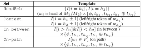
Set Template

HeadEmb {I[i=h1], I[i=h2]}

(wiis head ofM1/M2)⇥{ , th1, th2, th1 th2}

Context I[i=h1±1](left/right token ofwh1) I[i=h2±1](left/right token ofwh2)

In-between I[i > h1]&I[i < h2](in between )

⇥{ , th1, th2, th1 th2}

On-path I[wi2P](on path)

[image:5.595.308.536.61.142.2]

⇥{ , th1, th2, th1 th2}

Table 2: Feature sets used inFCM.

6 Experimental Settings

Features Our FCM features (Table 2) use a

fea-ture vector fwi over the word wi, the two

tar-get entities M1, M2, and their dependency path. Hereh1, h2 are the indices of the two head words ofM1, M2,⇥refers to the Cartesian product be-tween two sets,th1 andth2are entity types (named

entity tags for ACE 2005 or WordNet supertags for SemEval 2010) of the head words of two entities, and stands for the empty feature. refers to the conjunction of two elements. TheIn-between

features indicate whether a wordwiis in between

two target entities, and theOn-pathfeatures in-dicate whether the word is on the dependency path, on which there is a set of wordsP, between the two entities.

We also use the target entity type as a feature. Combining this with the basic features results in more powerful compound features, which can help us better distinguish the functions of word embed-dings for predicting certain relations. For exam-ple, if we have a person and a vehicle, we know it will be more likely that they have anART rela-tion. For theART relation, we introduce a corre-sponding weight vector, which is closer to lexical embeddings similar to the embedding of “drive”.

All linguistic annotations needed for fea-tures (POS, chunks7_{, parses) are from Stanford}

CoreNLP (Manning et al., 2014). Since SemEval does not have gold entity types we obtained Word-Net and named entity tags using Ciaramita and Altun (2006). For all experiments we use 200-d wor200-d embe200-d200-dings traine200-d on the NYT portion of the Gigaword 5.0 corpus (Parker et al., 2011), with word2vec (Mikolov et al., 2013). We use the CBOW model with negative sampling (15 nega-tive words). We set a window sizec=5, and re-move types occurring less than 5 times.

Models We consider several methods. (1) FCM

in isolation without fine-tuning. (2)FCM in

isola-tion with fine-tuning (i.e. trained as a log-bilinear

model). (3) A log-linear model with a rich binary feature set from Sun et al. (2011) (Baseline)— this consists of all the baseline features of Zhou et al. (2005) plus several additional carefully-chosen features that have been highly tuned for ACE-style relation extraction over years of research. We ex-clude the Country gazetteer and WordNet features from Zhou et al. (2005). The two remaining meth-ods are hybrid models that integrateFCMas a

sub-model within the log-linear sub-model (§4). We con-sider two combinations. (4) The feature set of Nguyen and Grishman (2014) obtained by using the embeddings of heads of two entity mentions (+HeadOnly). (5) Our full FCM model (+FCM).

All models use L2 regularization tuned on dev data.

6.1 Datasets and Evaluation

ACE 2005 We evaluate our relation extraction system on the English portion of the ACE 2005 corpus (Walker et al., 2006).8 _{There are 6}

do-mains: Newswire (nw), Broadcast Conversation (bc), Broadcast News (bn), Telephone Speech (cts), Usenet Newsgroups (un), and Weblogs (wl). Following prior work we focus on the do-main adaptation setting, where we train on one set (the union of the news domains (bn+nw), tune hyperparameters on a dev domain (half of bc) and evaluate on the remainder (cts, wl, and the remainder ofbc) (Plank and Moschitti, 2013; Nguyen and Grishman, 2014). We assume that gold entity spansandtypes are available for train and test. We use all pairs of entity mentions to yield 43,518 total relations in the training set. We report precision, recall, and F1 for relation extrac-tion. While it is not our focus, for completeness we include results with unknown entity types fol-lowing Plank and Moschitti (2013) (Appendix 1).

SemEval 2010 Task 8 We evaluate on the Se-mEval 2010 Task 8 dataset9 _{(Hendrickx et al.,}

2010) to compare with other compositional mod-els and highlight the advantages ofFCM. This task

is to determine the relation type (or no relation) between two entities in a sentence. We adopt the setting of Socher et al. (2012). We use 10-fold

8_{Many relation extraction systems evaluate on the ACE} 2004 corpus (Mitchell et al., 2005). Unfortunately, the most common convention is to use 5-fold cross validation, treating the entirety of the dataset as both trainandevaluation data. Rather than continuing to overfit this data by perpetuating the cross-validation convention, we instead focus on ACE 2005.

9_{http://docs.google.com/View?docid=dfvxd49s_36c28v9pmw}

cross validation on the training data to select hy-perparameters and do regularization by early stop-ping. The learning rates for FCM with/without

fine-tuning are 5e-3 and 5e-2 respectively. We report macro-F1 and compare to previously pub-lished results.

7 Results

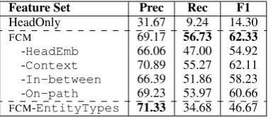
ACE 2005 DespiteFCM’s (1) simple feature set,

it is competitive with the log-linear baseline (3) on out-of-domain test sets (Table 3). In the typi-cal gold entity spans and types setting, both Plank and Moschitti (2013) and Nguyen and Grishman (2014) found that they were unable to obtain im-provements by adding embeddings to baseline fea-ture sets. By contrast, we find that on all do-mains the combination baseline +FCM(5) obtains

the highest F1 and significantly outperforms the other baselines,yielding the best reported results for this task. We found that fine-tuning of em-beddings (2) did not yield improvements on our out-of-domain development set, in contrast to our results below for SemEval. We suspect this is be-cause fine-tuning allows the model to overfit the training domain, which then hurts performance on the unseen ACE test domains. Accordingly, Ta-ble 3 shows only the log-linear model.

Finally, we highlight an important contrast be-tween FCM (1) and the log-linear model (3): the

latter uses over 50 feature templates based on a POS tagger, dependency parser, chunker, and con-stituency parser. FCM uses only a dependency

parse but still obtains better results (Avg. F1).

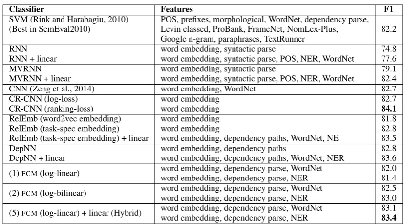
SemEval 2010 Task 8 Table 4 shows FCM

compared to the best reported results from the SemEval-2010 Task 8 shared task and several other compositional models.

For theFCMwe considered two feature sets. We

found that using NE tags instead of WordNet tags helps with fine-tuning but hurts without. This may be because the set of WordNet tags is larger mak-ing the model more expressive, but also introduces more parameters. When the embeddings are fixed, they can help to better distinguish different func-tions of embeddings. But when fine-tuning, it be-comes easier to over-fit. Alleviating over-fitting is a subject for future work (§9).

With either WordNet or NER features, FCM