WordRank: Learning Word Embeddings via Robust Ranking

WordRank

: Learning Word Embeddings via Robust Ranking

Shihao Ji

Parallel Computing Lab, Intel [email protected]

Hyokun Yun Amazon

[email protected]

Pinar Yanardag Purdue University [email protected]

Shin Matsushima University of Tokyo shin matsushima@mist.

i.u-tokyo.ac.jp

S. V. N. Vishwanathan Univ. of California, Santa Cruz

[email protected]

Abstract

Embedding words in a vector space has gained a lot of attention in recent years. While state-of-the-art methods provide efficient computa-tion of word similarities via a low-dimensional matrix embedding, their motivation is often left unclear. In this paper, we argue that word embedding can be naturally viewed as a rank-ingproblem due to the ranking nature of the evaluation metrics. Then, based on this in-sight, we propose a novel framework Wor-dRank that efficiently estimates word repre-sentations via robust ranking, in which the attention mechanism and robustness to noise are readily achieved via the DCG-like rank-ing losses. The performance ofWordRank is measured in word similarity and word anal-ogy benchmarks, and the results are com-pared to the state-of-the-art word embedding techniques. Our algorithm is very competi-tive to the state-of-the- arts on large corpora, while outperforms them by a significant mar-gin when the training set is limited (i.e., sparse and noisy). With 17 million tokens,WordRank performs almost as well as existing methods using 7.2 billion tokens on a popular word similarity benchmark. Our multi-node dis-tributed implementation ofWordRankis pub-licly available for general usage.

1 Introduction

Embedding words into a vector space, such that se-manticandsyntacticregularities between words are preserved, is an important sub-task for many appli-cations of natural language processing. Mikolov et al. (2013a) generated considerable excitement in the

machine learning and natural language processing communities by introducing a neural network based model, which they callword2vec. It was shown that

word2vecproduces state-of-the-art performance on both word similarity as well as word analogy tasks. The word similarity task is to retrieve words that are similar to a given word. On the other hand, word analogy requires answering queries of the form

a:b;c:?, wherea, b, andcare words from the vocab-ulary, and the answer to the query must be semanti-cally related tocin the same way as bis related to

a. This is best illustrated with a concrete example: Given the query king:queen;man:? we expect the model to outputwoman.

The impressive performance of word2vec led to a flurry of papers, which tried to explain and im-prove the performance of word2vec both theoreti-cally (Arora et al., 2015) and empiritheoreti-cally (Levy and Goldberg, 2014). One interpretation of word2vec

is that it is approximately maximizing the positive pointwise mutual information (PMI), and Levy and Goldberg (2014) showed that directly optimizing this gives good results. On the other hand, Penning-ton et al. (2014) showed performance comparable to

word2vec by using a modified matrix factorization model, which optimizes a log loss.

Somewhat surprisingly, Levy et al. (2015) showed that much of the performance gains of these new word embedding methods are due to certain hyper-parameter optimizations and system-design choices. In other words, if one sets up careful experiments, then existing word embedding models more or less perform comparably to each other. We conjecture that this is because, at a high level, all these methods

are based on the following template: From a large text corpus eliminate infrequent words, and compute a|W| × |C|word-context co-occurrence count ma-trix; a context is a word which appears less than d

distance away from a given word in the text, where

d is a tunable parameter. Let w ∈ W be a word andc ∈ C be a context, and letXw,c be the (poten-tially normalized) co-occurrence count. One learns a functionf(w, c)which approximates a transformed version ofXw,c. Different methods differ essentially

in the transformation function they use and the para-metric form of f (Levy et al., 2015). For exam-ple,GloVe(Pennington et al., 2014) usesf(w, c) = huw,vci whereuw andvc are k dimensional vec-tors, h·,_·i denotes the Euclidean dot product, and one approximatesf(w, c)≈logXw,c. On the other

hand, as Levy and Goldberg (2014) show,word2vec

can be seen as using the same f(w, c) as GloVe

but trying to approximatef(w, c) ≈ PMI(Xw,c)−

logn, where PMI(_·)is the pairwise mutual

informa-tion (Cover and Thomas, 1991) andnis the number of negative samples.

In this paper, we approach the word embedding task from a different perspective by formulating it as a ranking problem. That is, given a word

w, we aim to output an ordered list (c1, c2,· · ·)

of context words from C such that words that

co-occur with w appear at the top of the list. If

rank(w, c)denotes the rank ofcin the list, then

typ-ical ranking losses optimize the following objective:

P

(w,c)∈Ωρ(rank(w, c)), whereΩ⊂ W × C is the

set of word-context pairs that co-occur in the corpus, andρ(_·)is a ranking loss function that is

monotoni-cally increasing and concave (see Sec. 2 for a justi-fication).

Casting word embedding as ranking has two dis-tinctive advantages. First, our method is discrimina-tiverather than generative; in other words, instead of modeling (a transformation of)Xw,cdirectly, we only aim to model the relative order of Xw,· val-ues in each row. This formulation fits naturally to popular word embedding tasks such as word simi-larity/analogy since instead of the likelihood of each word, we are interested in finding the most relevant words in a given context1_{. Second, casting word}

1_{Roughly speaking, this difference in viewpoint is}

analo-gous to the difference between pointwise loss function vs

list-embedding as a ranking problem enables us to de-sign models robust to noise (Yun et al., 2014) and focusing more on differentiating top relevant words, a kind of attention mechanism that has been proved very useful in deep learning (Larochelle and Hin-ton, 2010; Mnih et al., 2014; Bahdanau et al., 2015). Both issues are very critical in the domain of word embedding since (1) the co-occurrence matrix might be noisy due to grammatical errors or unconven-tional use of language,i.e., certain words might co-occur purely by chance, a phenomenon more acute in smaller document corpora collected from diverse sources; and (2) it’s very challenging to sort out a few most relevant words from a very large vocabu-lary, thus some kind of attention mechanism that can trade off the resolution on most relevant words with the resolution on less relevant words is needed. We will show in the experiments that our method can mitigate some of these issues; with 17 million to-kens our method performs almost as well as existing methods using 7.2 billion tokens on a popular word similarity benchmark.

2 Word Embedding via Ranking

2.1 Notation

We usewto denote a word and cto denote a con-text. The set of all words, that is, the vocabulary is denoted asW and the set of all context words is

denotedC. We will useΩ _{⊂ W × C}to denote the

set of all word-context pairs that were observed in the data, Ωw to denote the set of contexts that co-occured with a given word w, and similarly Ωc to denote the words that co-occurred with a given con-textc. The size of a set is denoted as_|·|. The inner

product between vectors is denoted ash·,_·i.

2.2 Ranking Model

Let uw denote the k-dimensional embedding of a word w, and vc denote that of a context c. For convenience, we collect embedding parameters for words and contexts asU := _{uw}w∈W, andV :=

{vc}c∈C.

We aim to capture the relevance of context cfor

wordw by the inner product between their

We achieve this by learning a ranking model that is parametrized byUandV. If we sort the set of

con-textsCfor a given wordwin terms of each context’s

inner product score with the word, the rank of a spe-cific contextcin this list can be written as (Usunier

et al., 2009):

rank (w, c) =X

c0_∈C\{c}

I(_huw,vci − huw,vc0i ≤0)

=X

c0_∈C\{c}

I(_huw,vc−vc0i ≤0), (1)

whereI(x ≤0)is a 0-1 loss function which is 1 if

x _≤ 0 and0 otherwise. Since I(x _≤ 0)is a

dis-continuous function, we follow the popular strategy in machine learning which replaces the 0-1 loss by its convex upper bound`(<sub>·</sub>), where `(_·)can be any

popular loss function for binary classification such as the hinge loss`(x) = max (0,1−x)or the

lo-gistic loss `(x) = log₂(1 + 2−x) (Bartlett et al.,

2006). This enables us to construct the following convex upper bound on the rank:

rank (w, c)_≤rank (w, c)=X

c0_∈C\{c}

`(_huw,vc−vc0i) (2)

It is certainly desirable that the ranking model po-sitions relevant contexts at the top of the list; this motivates us to write the objective function to mini-mize as:

J(U,V):=X

w∈W

X

c∈Ωw

rw,c·ρ

rank (w, c)+β α

(3)

whererw,c is the weight between wordwand con-textcquantifying the association between them,ρ(·)

is a monotonically increasing and concave ranking loss function that measures goodness of a rank, and

α >0,β >0are the hyperparameters of the model

whose role will be discussed later. Following Pen-nington et al. (2014), we use

rw,c=

(

(Xw,c/xmax) ifXw,c < xmax

1 otherwise, (4)

where we setxmax = 100and = 0.75in our ex-periments. That is, we assign larger weights (with a saturation) to contexts that appear more often with the word of interest, and vice-versa. For the ranking

loss function ρ(·), on the other hand, we consider

the class of monotonically increasing and concave functions. While monotonicity is a natural require-ment, we argue that concavity is also important so that the derivative ofρis always non-increasing; this

implies that the ranking loss to be the most sensitive at the top of the list (where the rank is small) and becomes less sensitive at the lower end of the list (where the rank is high). Intuitively this is desir-able, because we are interested in a small number of relevant contexts which frequently co-occur with a given word, and thus are willing to tolerate errors on infrequent contexts2_{. Meanwhile, this insensitivity}

at the bottom of the list makes the model robust to noise in the data either due to grammatical errors or unconventional use of language. Therefore, a sin-gle ranking loss function ρ(_·) serves two different

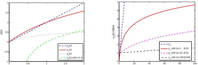
purposes at two ends of the curve (see the example plots of ρ in Figure 1); while the left hand side of

the curve encourages “high resolution” on most rel-evant words, the right hand side becomes less sen-sitive (with “low resolution”) to infrequent and pos-sibly noisy words3_{. As we will demonstrate in our}

experiments, this is a fundamental attribute (in addi-tion to the ranking nature) of our method that con-tributes its superior performance as compared to the state-of-the-arts when the training set is limited (i.e., sparse and noisy).

What are interesting loss functions that can be used forρ(·)? Here are four possible alternatives,

all of which have a natural interpretation (see the plots of all fourρ functions in Figure 1(a) and the

related work in Sec. 3 for a discussion).

ρ0(x) :=x (identity) (5)

ρ1(x) := log2(1 +x) (logarithm) (6)

ρ2(x) := 1− 1

log₂(2 +x) (negative DCG) (7)

ρ3(x) :=

x1−t−1

1₋t (logt witht6= 1) (8)

2_{This is similar to the attention mechanism found in human}

visual system that is able to focus on a certain region of an age with “high resolution” while perceiving the surrounding im-age in “low resolution” (Larochelle and Hinton, 2010; Mnih et al., 2014).

3_{Due to the linearity ofρ}

0 0.5 1 1.5 2 −1

−0.5 0 0.5 1 1.5 2

x

ρ

(x)

ρ0(x)

ρ1(x)

ρ2(x)

ρ3(x) with t=1.5

0 20 40 60 80 100 0

1 2 3 4 5 6 7

x

ρ1

((x+

β

)/

α

)

ρ0

ρ1 with (α=1, β=0)

ρ1 with (α=10, β=9)

ρ1 with (α=100,β=99)

Figure 1: (a) Visualizing different ranking loss functionsρ(x)as defined in Eqs. (5–8); the lower part ofρ3(x)is truncated in order to visualize the other functions better. (b) Visualizingρ1((x+β)/α)with differentαandβ;ρ0is included to illustrate the dramatic scale differences betweenρ0andρ1.

We will explore the performance of each of these variants in our experiments. For now, we turn our attention to efficient stochastic optimization of the objective function (3).

2.3 Stochastic Optimization

Plugging (2) into (3), and replacingP_w∈WP_c∈Ωw byP_(w,c)∈Ω, the objective function becomes:

J(U,V) = X

(w,c)∈Ω

rw,c·

ρ

P

c0_∈C\{c}`(huw,vc−vc0i)+β

α

!

. (9)

This function contains summations over Ω and C, both of which are expensive to compute for a large corpus. Although stochastic gradient descent (SGD) (Bottou and Bousquet, 2011) can be used to re-place the summation over Ω by random sampling,

the summation overCcannot be avoided unlessρ(_·)

is a linear function. To work around this problem, we propose to optimize a linearized upper bound of the objective function obtained through a first-order Taylor approximation. Observe that due to the con-cavity ofρ(_·), we have

ρ(x)≤ρ ξ−1+ρ0 ξ−1· x−ξ−1 (10)

for anyxandξ 6= 0. Moreover, the bound is tight

when ξ = x−1. This motivates us to introduce a

set of auxiliary parametersΞ := _{ξw,c}_(w,c)∈Ω and define the following upper bound ofJ(U,V):

J(U,V,Ξ) := X (w,c)∈Ω

rw,c·

(

ρ(ξ−_wc1) +ρ0(ξ_wc−1)_·

α−1β+α−1X

c0_∈C\{c}

`(_huw,vc−vc0i)−ξ−_w,c1

)

. (11)

Note thatJ(U,V) ≤ J(U,V,Ξ) for any Ξ, due

to (10)4_{. Also, minimizing (11) yields the sameU}

andVas minimizing (9). To see this, supposeUˆ := {uˆw}_w∈W andVˆ :={vˆc}_c∈C minimizes (9). Then, by letting_{Ξ :=}ˆ n_ξˆ_w,co

(w,c)∈Ωwhere

ˆ

ξw,c =

α

P

c0_∈C\{c}`(huˆw,vˆc−vˆc0i) +β, (12)

we have JUˆ,Vˆ,Ξˆ = JUˆ,Vˆ. Therefore,

it suffices to optimize (11). However, unlike (9), (11) admits an efficient SGD algorithm. To see this, rewrite (11) as

J(U,V,Ξ) =X (w,c,c0₎

rw,c·

ρ(ξ−1

w,c)+ρ0(ξ−w,c1)·(α−1β−ξw,c−1)

|C| −1

+ 1

αρ

0_(ξ−1

w,c)·`(huw,vc−vc0i)

!

, (13)

where(w, c, c0) _∈ Ω_×(_{C \ {}c_}). Then, it can be

seen that if we sample uniformly from(w, c) _∈ Ω

andc0∈ C \ {c}, thenj(w, c, c0) :=

|Ω|·(|C|−1)·rw,c·

ρ(ξ_w,c−1)+ρ0(ξ_w,c−1)_·(α−1β₋ξ_w,c−1) |C| −1

+ 1

αρ

0_(ξ−1

w,c)·`(huw,vc−vc0i)

!

, (14)

which does not contain any expensive summa-tions and is an unbiased estimator of (13), i.e.,

E[j(w, c, c0)] = J(U,V,Ξ). On the other hand,

one can optimizeξw,c exactly by using (12). Putting 4_Whenρ=ρ

0, one can simply set the auxiliary variables

everything together yields a stochastic optimiza-tion algorithm WordRank, which can be special-ized to a variety of ranking loss functionsρ(·)with

weights rw,c (e.g., DCG (Discounted Cumulative Gain) (Manning et al., 2008) is one of many pos-sible instantiations). Algorithm 1 contains detailed pseudo-code. It can be seen that the algorithm is di-vided into two stages: a stage that updates(U,V)

and another that updatesΞ. Note that the time com-plexity of the first stage isO(|Ω|)since the cost of

each update in Lines 8–10 is independent of the size of the corpus. On the other hand, the time complex-ity of updating Ξ in Line 15 is O(|Ω| |C|), which

can be expensive. To amortize this cost, we em-ploy two tricks: we only update Ξ after a few it-erations ofUandVupdate, and we exploit the fact

that the most computationally expensive operation in (12) involves a matrix and matrix multiplication which can be calculated efficiently via the SGEMM routine in BLAS (Dongarra et al., 1990).

Algorithm 1WordRankalgorithm. 1: η: step size

2: repeat

3: // Stage 1: Update U and V

4: repeat

5: Sample(w, c)uniformly fromΩ 6: Samplec0uniformly from_{C \ {}c_}

7: // following three updates

are executed simultaneously

8: uw ← uw − η · rw,c · ρ0(ξw,c−1) ·

`0(huw,vc−vc0i)·(vc−vc0)

9: vc ← vc − η · rw,c · ρ0(ξw,c−1) ·

`0(_huw,vc−vc0i)·uw

10: v_c0 ← v_c0 + η · rw,c · ρ0(ξ−w,c1) ·

`0(huw,vc−vc0i)·u_w 11: untilUandVare converged

12: // Stage 2: Update Ξ

13: forw∈ W do

14: forc_{∈ C}do

15: ξw,c=α/P_c0_∈C\{c}`(huw,vc−vc0i)+β

16: end for

17: end for

18: untilU,VandΞare converged

2.4 Parallelization

The updates in Lines 8–10 have one remarkable property: To updateuw,vc andvc0, we only need toreadthe variablesuw,vc,vc0 andξw,c. What this means is that updates to another triplet of variables

uw,ˆ vˆc and v_cˆ0 can be performed independently. This observation is the key to developing a parallel optimization strategy, by distributing the computa-tion of the updates among multiple processors. Due to lack of space, details including pseudo-code are relegated to the supplementary material.

2.5 Interpreting ofαandβ

The update (12) indicates that ξ−_w,c1 is proportional

torank (w, c). On the other hand, one can observe that the loss function`(·)in (14) is weighted by a

ρ0 ξ−1

w,c

term. Since ρ(_·) is concave, its gradient

ρ0(_·)is monotonically non-increasing (Rockafellar, 1970). Consequently, whenrank (w, c) and hence

ξ_w,c−1 is large, ρ0 ξ_w,c−1is small. In other words, the

loss function “gives up” on contexts with high ranks in order to focus its attention on top of the list. The rate at which the algorithm gives up is determined by the hyperparametersαandβ. For the illustration of this effect, see the example plots ofρ1 with

dif-ferentαandβ in Figure 1(b). Intuitively,αcan be

viewed as ascaleparameter whileβ can be viewed as anoffsetparameter. An equivalent interpretation is that by choosing different values ofα andβ one

can modify the behavior of the ranking lossρ(_·)in a problem dependent fashion. In our experiments, we found that a common setting ofα= 1andβ= 0

of-ten yields uncompetitive performance, while setting

α= 100andβ= 99generally gives good results.

3 Related Work

Our work sits at the intersection of word embed-ding and ranking optimization. As we discussed in Sec. 2.2 and Sec. 2.5, it’s also related to the atten-tion mechanism widely used in deep learning. We therefore review the related work along these three axes.

Word Embedding. We already discussed some related work (word2vec and GloVe) on word em-bedding in the introduction. Essentially, word2vec

WordRank learns word representations via robust ranking. Besides these state-of-the-art techniques, a few ranking-based approaches have been proposed for word embedding recently, e.g., (Collobert and Weston, 2008; Vilnis and McCallum, 2015; Liu et al., 2015). However, all of them adopt a pair-wise binary classification approach with a linear rank-ing loss ρ0. For example, (Collobert and Weston,

2008; Vilnis and McCallum, 2015) employ a hinge loss on positive/negative word pairs to learn word representations andρ0is usedimplicitlyto evaluate

ranking losses. As we discussed in Sec. 2.2,ρ0has

no benefit of the attention mechanism and robust-ness to noise since its linearity treats all the rank-ing errors uniformly; empirically, sub-optimal per-formances are often observed withρ0 in our

exper-iments. More recently, by extending the Skip-Gram model of word2vec, Liu et al. (2015) incorporates additional pair-wise constraints induced from 3rd-party knowledge bases, such as WordNet, and learns word representations jointly. In contrast,WordRank

is a fully ranking-based approach without using any additional data source for training.

Robust Ranking. The second line of work that is very relevant toWordRankis that of ranking objec-tive (3). The use of score functions huw,vci for ranking is inspired by the latent collaborative re-trieval framework of Weston et al. (2012). Writing the rank as a sum of indicator functions (1), and upper bounding it via a convex loss (2) is due to Usunier et al. (2009). Usingρ0(·) (5) corresponds

to the well-known pairwise ranking loss (see e.g., (Lee and Lin, 2013)). On the other hand, Yun et al. (2014) observed that if they set ρ = ρ2 as in

(7), then−J(U,V)corresponds to the DCG

(Dis-counted Cumulative Gain), one of the most popular ranking metrics used in web search ranking (Man-ning et al., 2008). In their RobiRank algorithm they proposed the use ofρ = ρ1 (6), which they

consid-ered to be a special function for which one can de-rive an efficient stochastic optimization procedure. However, as we showed in this paper, the general class of monotonically increasing concave functions can be handled efficiently. Another important differ-ence of our approach is the hyperparametersα and β, which we use to modify the behavior of ρ, and

which we find are critical to achieve good empirical

results. Ding and Vishwanathan (2010) proposed the use ofρ= log_tin the context of robustbinary

classi-fication, while here we are concerned with ranking, and our formulation is very general and applies to a variety of ranking lossesρ(_·)with weightsrw,c. Op-timizing overUandVby distributing the

computa-tion across processors is inspired by work on dis-tributed stochastic gradient for matrix factorization (Gemulla et al., 2011).

Attention. Attention is one of the most impor-tant advancements in deep learning in recent years (Larochelle and Hinton, 2010), and is now widely used in state-of-the-art image recognition and ma-chine translation systems (Mnih et al., 2014; Bah-danau et al., 2015). Recently, attention has also been applied to the domain of word embedding. For ex-ample, under the intuition that not all contexts are created equal, Wang et al. (2015) assign an impor-tance weight to each word type at each context po-sition and learn an attention-based Continuous Bag-Of-Words (CBOW) model. Similarly, within a rank-ing framework,WordRankexpresses the context im-portance by introducing the auxiliary variableξw,c,

which “gives up” on contexts with high ranks in or-der to focus its attention on top of the list.

4 Experiments

In our experiments, we first evaluate the impact of the weight rw,c and the ranking loss function ρ(·) on the test performance using a small dataset. We then pick the best performing model and compare it againstword2vec(Mikolov et al., 2013b) andGloVe

(Pennington et al., 2014). We closely follow the framework of Levy et al. (2015) to set up a careful and fair comparison of the three methods. Our code is publicly available at https://bitbucket.

org/shihaoji/wordrank.

Training Corpus Models are trained on a com-bined corpus of 7.2 billion tokens, which consists of the 2015 Wikipedia dump with 1.6 billion tokens, the WMT14 News Crawl5 _{with 1.7 billion tokens,}

the “One Billion Word Language Modeling Bench-mark”6 _{with almost 1 billion tokens, and UMBC}

5_{http://www.statmt.org/wmt14/}

translation-task.html

Corpus Size 17M∗ _{32M 64M 128M 256M 512M 1.0B 1.6B 7.2B} Vocabulary Size|W| 71K 100K 100K 200K 200K 300K 300K 400K 620K

Window Sizewin 15 15 15 10 10 10 10 10 10

Dimensionk 100 100 100 200 200 300 300 300 300

* This is the Text8 dataset fromhttp://mattmahoney.net/dc/text8.zip, which is widely used for word embedding demo.

Table 1:Parameter settings used in the experiments.

Task Robi ρ0 ρ1 ρ2 ρ3

off on off on off on off on

Similarity 41.2 69.0 71.0 66.7 70.4 66.8 70.8 68.1 68.0 Analogy 22.7 24.9 31.9 34.3 44.5 32.3 40.4 33.6 42.9

Table 2:Performance of differentρfunctions on Text8 dataset with 17M tokens.

webbase corpus7_{with around 3 billion tokens. The}

pre-processing pipeline breaks the paragraphs into sentences, tokenizes and lowercases each corpus with the Stanford tokenizer. We further clean up the dataset by removing non-ASCII characters and punctuation, and discard sentences that are shorter than 3 tokens or longer than 500 tokens. In the end, we obtain a dataset of 7.2 billion tokens, with the first 1.6 billion tokens from Wikipedia. When we want to experiment with a smaller corpus, we ex-tract a subset which contains the specified number of tokens.

Co-occurrence matrix construction We use the

GloVe code to construct the co-occurrence matrix

X, and the same matrix is used to trainGloVe and

WordRankmodels. When constructingX, we must

choose the size of the vocabulary, the context win-dow and whether to distinguish left context from right context. We follow the findings and design choices of GloVe and use a symmetric window of size win with a decreasing weighting function, so

that word pairs that aredwords apart contribute1/d

to the total count. Specifically, when the corpus is small (e.g., 17M, 32M, 64M) we let win= 15 and

for larger corpora we letwin= 10. The larger

win-dow size alleviates the data sparsity issue for small corpus at the expense of adding more noise to X.

The parameter settings used in our experiments are summarized in Table 1.

Using the trained model It has been shown by Pennington et al. (2014) that combining theuw and

vc vectors with equal weights gives a small boost

7_{http://ebiquity.umbc.edu/resource/html/}

id/351

in performance. This vector combination was origi-nally motivated as an ensemble method (Pennington et al., 2014), and later Levy et al. (2015) provided a different interpretation of its effect on the cosine similarity function, and show that adding context vectors effectively adds first-order similarity terms to the second-order similarity function. In our ex-periments, we find that vector combination boosts the performance in word analogy task when training set is small, but when dataset is large enough (e.g., 7.2 billion tokens), vector combination doesn’t help anymore. More interestingly, for the word similarity task, we find that vector combination is detrimen-tal in all the cases, sometimes even substantially8_.

Therefore, we will always useuwon word similarity task, and useuw +vcon word analogy task unless otherwise noted.

4.1 Evaluation

Word Similarity We use six datasets to evaluate word similarity: WS-353 (Finkelstein et al., 2002) partitioned into two subsets: WordSim Similarity and WordSim Relatedness (Agirre et al., 2009); MEN (Bruni et al., 2012); Mechanical Turk (Radin-sky et al., 2011); Rare words (Luong et al., 2013); and SimLex-999 (Hill et al., 2014). They contain word pairs together with human-assigned similarity judgments. The word representations are evaluated by ranking the pairs according to their cosine simi-larities, and measuring the Spearman’s rank correla-tion coefficient with the human judgments.

8_{This is possible since we optimize a ranking loss: the}

ab-solute scores don’t matter as long as they yield an ordered list correctly. Thus, WordRank’suw and vc are less comparable

Word Analogies For this task, we use the Google analogy dataset (Mikolov et al., 2013a). It contains 19544 word analogy questions, partitioned into 8869 semantic and 10675 syntactic questions. A question is correctly answered only if the algorithm selects the word that is exactly the same as the correct word in the question: synonyms are thus counted as mis-takes. There are two ways to answer these questions, namely, by using 3CosAdd or 3CosMul (see (Levy and Goldberg, 2014) for details). We will report scores by using 3CosAdd by default, and indicate when 3CosMul gives better performance.

4.2 The impact ofrw,candρ(·)

In Sec. 2.2 we argued the need for adding weight

rw,c to ranking objective (3), and we also presented our framework which can deal with a variety of ranking loss functions ρ. We now study the utility of these two ideas. We report results on the 17 mil-lion token dataset in Table 2. For the similarity task, we use the WS-353 test set and for the analogy task we use the Google analogy test set. The best scores for each task are underlined. We sett= 1.5forρ3.

“Off” means that we used uniform weightrw,c= 1, and “on” means thatrw,cwas set as in (4). For com-parison, we also include the results using RobiRank (Yun et al., 2014)9_.

It can be seen from Table 2 that adding the weight

rw,c improves performance in all the cases, espe-cially on the word analogy task. Among the four

ρfunctions,ρ0 performs the best on the word

simi-larity task but suffers notably on the analogy task, while ρ1 = log performs the best overall. Given

these observations, which are consistent with the re-sults on large scale datasets, in the experiments that follow we only reportWordRankwith the best con-figuration,i.e., using ρ1 with the weightrw,c as de-fined in (4).

4.3 Comparison to state-of-the-arts

In this section we compare the performance of Wor-dRank with word2vec10 _{and GloVe}11_{, by using the}

9_{We used the code provided by the authors athttps://}

bitbucket.org/d_ijk_stra/robirank. Although

related to RobiRank, we attribute the superior performance of WordRankto the use of weightrw,c(4), introduction of

hyper-parametersαandβ, and many implementation details.

10_{https://code.google.com/p/word2vec/}

11_{http://nlp.stanford.edu/projects/glove}

code provided by the respective authors. For a fair comparison, GloVe andWordRank are given as in-put the same co-occurrence matrix X; this

elimi-nates differences in performance due to window size and other such artifacts, and the same parameters are used toword2vec. Moreover, the embedding di-mensions used for each of the three methods is the same (see Table 1). With word2vec, we train the Skip-Gram with Negative Sampling (SGNS) model since it produces state-of-the-art performance, and is widely used in the NLP community (Mikolov et al., 2013b). ForGloVe, we use the default parame-ters as suggested by (Pennington et al., 2014). The results are provided in Figure 2 (also see Table 4 in the supplementary material for additional details).

As can be seen, when the size of corpus increases, in general all three algorithms improve their predic-tion accuracy on both tasks. This is to be expected since a larger corpus typically produces better statis-tics and less noise in the co-occurrence matrix X.

When the corpus size is small (e.g., 17M, 32M, 64M, 128M),WordRankyields the best performance with significant margins among three, followed by

word2vec and GloVe; when the size of corpus in-creases further, on the word analogy taskword2vec

andGloVe become very competitive to WordRank, and eventually perform neck-to-neck to each other (Figure 2(b)). This is consistent with the findings of (Levy et al., 2015) indicating that when the number of tokens is large even simple algorithms can per-form well. On the other hand, WordRank is dom-inant on the word similarity task for all the cases (Figure 2(a)) since it optimizes a ranking loss explic-itly, which aligns more naturally with the objective of word similarity than the other methods; with 17 million tokens our method performs almost as well as existing methods using 7.2 billion tokens on the word similarity benchmark.

17M 32M 64M 128M 256M 512M 1B 1.6B 7.2B 45

50 55 60 65 70 75 80

Number of Tokens

Accuracy [%]

Word2Vec GloVe WordRank

17M 32M 64M 128M 256M 512M 1B 1.6B 7.2B 30

35 40 45 50 55 60 65 70 75 80

Number of Tokens

Accuracy [%]

Word2Vec GloVe WordRank

Figure 2: Performance evolution as a function of corpus size (a) on WS-353 word similarity benchmark; (b) on Google word analogy benchmark.

Word Similarity Word Analogy

Model WordSim WordSim Bruni et Radinsky Luong et Hill et al. Goog Goog Similarity Relatedness al. MEN et al. MT al. RW SimLex Sem. Syn.

word2vec 73.9 60.9 75.4 66.4 45.5 36.6 78.8 72.0

GloVe 75.7 67.5 78.8 69.7 43.6 41.6 80.9 71.1

WordRank 79.4 70.5 78.1 73.5 47.4 43.5 78.4 74.7

Table 3:Performance of the bestword2vec,GloVeandWordRankmodels, learned from 7.2 billion tokens, on six similarity tasks and Google semantic and syntactic subtasks.

5 Visualizing the results

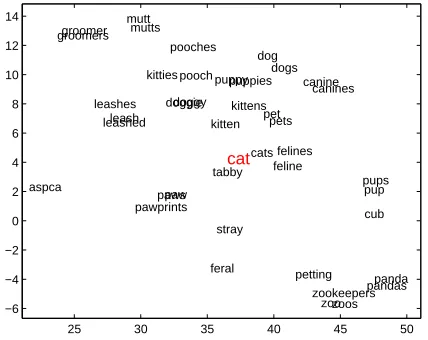
To understand whether WordRankproduces syntat-ically and semantically meaningful vector space, we did the following experiment: we use the best performing model produced using 7.2 billion to-kens, and compute the nearest neighbors of the word “cat”. We then visualize the words in two dimen-sions by using t-SNE (Maaten and Hinton, 2008). As can be seen in Figure 3, our ranking-based model is indeed capable of capturing both semantic (e.g., cat, feline, kitten, tabby) and syntactic (e.g., leash, leashes, leashed) regularities of the English lan-guage.

6 Conclusion

We proposedWordRank, a ranking-based approach, to learn word representations from large scale tex-tual corpora. The most prominent difference be-tween our method and the state-of-the-art tech-niques, such as word2vec and GloVe, is that Wor-dRanklearns word representations via a robust rank-ing model, while word2vec and GloVe typically model a transformation of co-occurrence countXw,c directly. Moreover, by a ranking loss functionρ(·), WordRankachieves its attention mechanism and ro-bustness to noise naturally, which are usually

lack-25 30 35 40 45 50 −6

−4 −2 0 2 4 6 8 10 12 14

cats feline kitten

felines dog

pet dogs

kittens pets

tabby paws

canine puppypuppies pooch doggie

canines

pups kitties

pup paw

leashed

feral pawprints

zoo doggy

pooches

aspca

zoos cub mutts

petting stray

zookeepers groomers

leash

panda groomer

pandas leashes

mutt

cat

Figure 3: Nearest neighbors of “cat” found by projecting a 300d word embedding learned fromWordRankonto a 2d space.

ing in other ranking-based approaches. These at-tributes significantly boost the performance of Wor-dRankin the cases where training data are sparse and noisy. Our multi-node distributed implementation of

WordRankis publicly available for general usage.

Acknowledgments

References

Eneko Agirre, Enrique Alfonseca, Keith Hall, Jana Kravalova, Marius Pasca, and Aitor Soroa. 2009. A study on similarity and relatedness using distributional and wordnet-based approaches. Proceedings of Hu-man Language Technologies, pages 19–27.

Sanjeev Arora, Yuanzhi Li, Yingyu Liang, Tengyu Ma, and Andrej Risteski. 2015. Random walks on context spaces: Towards an explanation of the mysteries of se-mantic word embeddings. Technical report, ArXiV.

http://arxiv.org/pdf/1502.03520.pdf.

Dzmitry Bahdanau, Kyunghyun Cho, and Yoshua Ben-gio. 2015. Neural machine translation by jointly learning to align and translate. In Proceedings of the International Conference on Learning Represen-tations (ICLR).

Peter L. Bartlett, Michael I. Jordan, and Jon D. McAuliffe. 2006. Convexity, classification, and risk bounds. Journal of the American Statistical Associa-tion, 101(473):138–156.

L´eon Bottou and Olivier Bousquet. 2011. The trade-offs of large-scale learning.Optimization for Machine Learning, page 351.

Elia Bruni, Gemma Boleda, Marco Baroni, and Nam Khanh Tran. 2012. Distributional semantics in technicolor. Proceedings of the 50th Annual Meet-ing of the Association for Computational LMeet-inguistics, pages 136–145.

Ronan Collobert and Jason Weston. 2008. A unified ar-chitecture for natural language processing: Deep neu-ral networks with multitask learning. InProceedings of the 25th international conference on Machine learn-ing, pages 160–167. ACM.

T. M. Cover and J. A. Thomas. 1991. Elements of Infor-mation Theory. John Wiley and Sons, New York. Nan Ding and S. V. N. Vishwanathan. 2010.t-logistic

re-gression. In Richard Zemel, John Shawe-Taylor, John Lafferty, Chris Williams, and Alan Culota, editors, Ad-vances in Neural Information Processing Systems 23. J. J. Dongarra, J. Du Croz, S. Duff, and S. Hammarling.

1990. A set of level 3 basic linear algebra subpro-grams. ACM Transactions on Mathematical Software, 16:1–17.

Lev Finkelstein, Evgeniy Gabrilovich, Yossi Matias, Ehud Rivlin, Zach Solan, Gadi Wolfman, and Eytan Ruppin. 2002. Placing search in context: The concept revisited. ACM Transactions on Information Systems, 20:116–131.

R. Gemulla, E. Nijkamp, P. J. Haas, and Y. Sisma-nis. 2011. Large-scale matrix factorization with dis-tributed stochastic gradient descent. InConference on Knowledge Discovery and Data Mining, pages 69–77.

Felix Hill, Roi Reichart, and Anna Korhonen. 2014. Simlex-999: Evaluating semantic models with (gen-uine) similarity estimation. Proceedings of the Sev-enteenth Conference on Computational Natural Lan-guage Learning.

Hugo Larochelle and Geoffrey E. Hinton. 2010. Learn-ing to combine foveal glimpses with a third-order boltzmann machine. InAdvances in Neural Informa-tion Processing Systems (NIPS) 23, pages 1243–1251. Ching-Pei Lee and Chih-Jen Lin. 2013. Large-scale

lin-ear ranksvm. Neural Computation. To Appear. Omer Levy and Yoav Goldberg. 2014. Neural word

embedding as implicit matrix factorization. In Max Welling, Zoubin Ghahramani, Corinna Cortes, Neil Lawrence, and Kilian Weinberger, editors, Advances in Neural Information Processing Systems 27, pages 2177–2185.

Omer Levy, Yoav Goldberg, and Ido Dagan. 2015. Im-proving distributional similarity with lessons learned from word embeddings. Transactions of the Associa-tion for ComputaAssocia-tional Linguistics, 3:211–225. Quan Liu, Hui Jiang, Si Wei, Zhen-Hua Ling, and Yu Hu.

2015. Learning semantic word embeddings based on ordinal knowledge constraints. InProceedings of the Annual Meeting of the Association for Computational Linguistics (ACL), pages 1501–1511.

Minh-Thang Luong, Richard Socher, and Christopher D. Manning. 2013. Better word representations with re-cursive neural networks for morphology. Proceedings of the Seventeenth Conference on Computational Nat-ural Language Learning, pages 104–113.

L. van der Maaten and G.E. Hinton. 2008. Visualizing high-dimensional data using t-sne. jmlr, 9:2579–2605. C. D. Manning, P. Raghavan, and H. Sch¨utze. 2008. In-troduction to Information Retrieval. Cambridge Uni-versity Press.

Tomas Mikolov, Kai Chen, Greg Corrado, and Jeffrey Dean. 2013a. Efficient estimation of word representa-tions in vector space.arXiv preprint arXiv:1301.3781. Tomas Mikolov, Ilya Sutskever, Kai Chen, Greg Cor-rado, and Jeffrey Dean. 2013b. Distributed represen-tations of words and phrases and their composition-ality. In Chris Burges, Leon Bottou, Max Welling, Zoubin Ghahramani, and Kilian Weinberger, editors, Advances in Neural Information Processing Systems 26.

Volodymyr Mnih, Nicolas Heess, Alex Graves, and Ko-ray Kavukcuoglu. 2014. Recurrent models of visual attention. InAdvances in Neural Information Process-ing Systems (NIPS) 27, pages 2204–2212.

Kira Radinsky, Eugene Agichtein, Evgeniy Gabrilovich, and Shaul Markovitch. 2011. A word at a time: Com-puting word relatedness using temporal semantic anal-ysis. Proceedings of the 20th international conference on World Wide Web, pages 337–346.

R. T. Rockafellar. 1970. Convex Analysis, volume 28 of Princeton Mathematics Series. Princeton University Press, Princeton, NJ.

Nicolas Usunier, David Buffoni, and Patrick Gallinari. 2009. Ranking with ordered weighted pairwise clas-sification. InProceedings of the International Confer-ence on Machine Learning.

Luke Vilnis and Andrew McCallum. 2015. Word repre-sentations via gaussian embedding. InProceedings of the International Conference on Learning Representa-tions (ICLR).

Ling Wang, Chu-Cheng Lin, Yulia Tsvetkov, Silvio Amir, Ramon Fernandez Astudillo, Chris Dyer, Alan Black, and Isabel Trancoso. 2015. Not all contexts are cre-ated equal: Better word representations with variable attention. InEMNLP.

Jason Weston, Chong Wang, Ron Weiss, and Adam Berenzweig. 2012. Latent collaborative retrieval. arXiv preprint arXiv:1206.4603.