Word Sense Discrimination by Clustering Contexts in Vector and Similarity Spaces

Word Sense Discrimination by Clustering Contexts

in Vector and Similarity Spaces

Amruta Purandare and Ted Pedersen

Department of Computer Science

University of Minnesota

Duluth, MN 55812 USA

{

pura0010,tpederse

}

@d.umn.edu

http://senseclusters.sourceforge.net

Abstract

This paper systematically compares unsuper-vised word sense discrimination techniques that cluster instances of a target word that oc-cur in raw text using both vector and similarity spaces. The context of each instance is repre-sented as a vector in a high dimensional fea-ture space. Discrimination is achieved by clus-tering these context vectors directly in vector space and also by finding pairwise similarities among the vectors and then clustering in sim-ilarity space. We employ two different repre-sentations of the context in which a target word occurs. First order context vectors represent the context of each instance of a target word as a vector of features that occur in that con-text. Second order context vectors are an indi-rect representation of the context based on the average of vectors that represent the words that occur in the context. We evaluate the discrim-inated clusters by carrying out experiments us-ing sense–tagged instances of 24 SENSEVAL -2 words and the well known Line, Hard and

Serve sense–tagged corpora.

1

Introduction

Most words in natural language have multiple possible meanings that can only be determined by considering the context in which they occur. Given a target word used in a number of different contexts, word sense dis-crimination is the process of grouping these instances of the target word together by determining which contexts are the most similar to each other. This is motivated by (Miller and Charles, 1991), who hypothesize that words with similar meanings are often used in similar contexts. Hence, word sense discrimination reduces to the problem of finding classes of similar contexts such that each class

represents a single word sense. Put another way, contexts that are grouped together in the same class represent a particular word sense.

While there has been some previous work in sense dis-crimination (e.g., (Sch¨utze, 1992), (Pedersen and Bruce, 1997), (Pedersen and Bruce, 1998), (Sch¨utze, 1998), (Fukumoto and Suzuki, 1999)), by comparison it is much less than that devoted to word sense disambiguation, which is the process of assigning a meaning to a word from a predefined set of possibilities. However, solutions to disambiguation usually require the availability of an external knowledge source or manually created sense– tagged training data. As such these are knowledge inten-sive methods that are difficult to adapt to new domains.

By contrast, word sense discrimination is an unsuper-vised clustering problem. This is an attractive methodol-ogy because it is a knowledge lean approach based on ev-idence found in simple raw text. Manually sense tagged text is not required, nor are specific knowledge rich re-sources like dictionaries or ontologies. Instances are clus-tered based on their mutual contextual similarities which can be completely computed from the text itself.

This paper presents a systematic comparison of dis-crimination techniques suggested by Pedersen and Bruce ((Pedersen and Bruce, 1997), (Pedersen and Bruce, 1998)) and by Sch¨utze ((Sch¨utze, 1992), (Sch¨utze, 1998)). This paper also proposes and evaluates several extensions to these techniques.

2

Previous Work

(Pedersen and Bruce, 1997) and (Pedersen and Bruce, 1998) propose a (dis)similarity based discrimination ap-proach that computes (dis)similarity among each pair of instances of the target word. This information is recorded in a (dis)similarity matrix whose rows/columns repre-sent the instances of the target word that are to be dis-criminated. The cell entries of the matrix show the de-gree to which the pair of instances represented by the corresponding row and column are (dis)similar. The (dis)similarity is computed from the first order context

vectors of the instances which show each instance as a

vector of features that directly occur near the target word in that instance.

(Sch¨utze, 1998) introduces second order context

vec-tors that represent an instance by averaging the feature

vectors of the content words that occur in the context of the target word in that instance. These second order con-text vectors then become the input to the clustering algo-rithm which clusters the given contexts in vector space, instead of building the similarity matrix structure.

There are some significant differences in the ap-proaches suggested by Pedersen and Bruce and by Sch¨utze. As yet there has not been any systematic study to determine which set of techniques results in better sense discrimination. In the sections that follow, we high-light some of the differences between these approaches.

2.1 Context Representation

Pedersen and Bruce represent the context of each test in-stance as a vector of features that directly occur near the target word in that instance. We refer to this representa-tion as the first order context vector. Sch¨utze, by contrast, uses the second order context representation that averages the first order context vectors of individual features that occur near the target word in the instance. Thus, Sch¨utze represents each feature as a vector of words that occur in its context and then computes the context of the target word by adding the feature vectors of significant content words that occur near the target word in that context.

2.2 Features

Pedersen and Bruce use a small number of local features that include co–occurrence and part of speech informa-tion near the target word. They select features from the same test data that is being discriminated, which is a com-mon practice in clustering in general. Sch¨utze represents contexts in a high dimensional feature space that is cre-ated using a separate large corpus (referred to as the train-ing corpus). He selects features based on their frequency counts or log-likelihood ratios in this corpus.

In this paper, we adopt Sch¨utze’s approach and select features from a separate corpus of training data, in part because the number of test instances may be relatively

small and may not be suitable for selecting a good feature set. In addition, this makes it possible to explore varia-tions in the training data while maintaining a consistent test set. Since the training data used in unsupervised clus-tering does not need to be sense tagged, in future work we plan to develop methods of collecting very large amounts of raw corpora from the Web and other online sources and use it to extract features.

Sch¨utze represents each feature as a vector of words that co–occur with that feature in the training data. These feature vectors are in fact the first order context vectors of the feature words (and not target word). The words that co–occur with the feature words form the dimensions of the feature space. Sch¨utze reduces the dimensional-ity of this feature space using Singular Value Decompo-sition (SVD), which is also employed by related tech-niques such as Latent Semantic Indexing (Deerwester et al., 1990) and Latent Semantic Analysis (Landauer et al., 1998). SVD has the effect of converting a word level feature space into a concept level semantic space that smoothes the fine distinctions between features that rep-resent similar concepts.

2.3 Clustering Space

Pedersen and Bruce represent instances in a (dis)similarity space where each instance can be seen as a point and the distance between any two points is a func-tion of their mutual (dis)similarities. The (dis)similarity matrix showing the pair-wise (dis)similarities among the instances is given as the input to the agglomerative clustering algorithm. The context group discrimination method used by Sch¨utze, on the other hand, operates on the vector representations of instances and thus works in vector space. Also he employs a hybrid clustering approach which uses both an agglomerative and the Estimation Maximization (EM) algorithm.

3

First Order Context Vectors

First order context vectors directly indicate which fea-tures make up a context. In all of our experiments, the context of the target word is limited to 20 surrounding content words on either side. This is true both when we are selecting features from a set of training data, or when we are converting test instances into vectors for cluster-ing. The particular features we are interested in are bi-grams and co–occurrences.

the training data, and the two words must have a log– likelihood ratio in excess of 3.841, which has the effect of removing co–occurrences and bigrams that have more than 95% chance of being independent of the target word. After selecting a set of co-occurrences or bigrams from a corpus of training data, a first order context representa-tion is created for each test instance. This shows how many times each feature occurs in the context of the tar-get word (i.e., within 20 positions from the tartar-get word) in that instance.

4

Second Order Context Vectors

A test instance can be represented by a second order con-text vector by finding the average of the first order concon-text vectors that are associated with the words that occur near the target word. Thus, the second order context represen-tation relies on the first order context vectors of feature words. The second order experiments in this paper use two different types of features, co–occurrences and bi-grams, defined as they are in the first order experiments.

Each co–occurrence identified in training data is as-signed a unique index and occupies the corresponding row/column in a word co–occurrence matrix. This is constructed from the co–occurrence pairs, and is a sym-metric adjacency matrix whose cell values show the log-likelihood ratio for the pair of words representing the corresponding row and column. Each row of the co– occurrence matrix can be seen as a first order context vec-tor of the word represented by that row. The set of words forming the rows/columns of the co–occurrence matrix are treated as the feature words.

Bigram features lead to a bigram matrix such that for each selected bigram WORDi<>WORDj, WORDi represents a single row, say the ith row, and WORDj represents a single column, say the jth column, of the bigram matrix. Then the value of cell (i,j) indi-cates the log–likelihood ratio of the words in the bigram WORDi<>WORDj. Each row of the bigram matrix can be seen as a bigram vector that shows the scores of all bigrams in which the word represented by that row oc-curs as the first word. Thus, the words representing the rows of the bigram matrix make the feature set while the words representing the columns form the dimensions of the feature space.

5

Clustering

The objective of clustering is to take a set of instances represented as either a similarity matrix or context vec-tors and cluster together instances that are more like each other than they are to the instances that belong to other clusters.

Clustering algorithms are classified into three main categories, hierarchical, partitional, and hybrid methods

that incorporate ideas from both. The algorithm acts as a search strategy that dictates how to proceed through the instances. The actual choice of which clusters to split or merge is decided by a criteria function. This section describes the clustering algorithms and criteria functions that have been employed in our experiments.

5.1 Hierarchical

Hierarchical algorithms are either agglomerative or divi-sive. They both proceed iteratively, and merge or divide clusters at each step. Agglomerative algorithms start with each instance in a separate cluster and merge a pair of clusters at each iteration until there is only a single clus-ter remaining. Divisive methods start with all instances in the same cluster and split one cluster into two during each iteration until all instances are in their own cluster.

The most widely known criteria functions used with hi-erarchical agglomerative algorithms are single link, com-plete link, and average link, also known as UPGMA. (Sch¨utze, 1998) points out that single link clustering tends to place all instances into a single elongated clus-ter, whereas (Pedersen and Bruce, 1997) and (Purandare, 2003) show that hierarchical agglomerative clustering using average link (via McQuitty’s method) fares well. Thus, we have chosen to use average link/UPGMA as our criteria function for the agglomerative experiments.

In similarity space, each instance can be viewed as a node in a weighted graph. The weights on edges joining two nodes indicate their pairwise similarity as measured by the cosine between the context vectors that represent the pair of instances.

When agglomerative clustering starts, each node is in its own cluster and is considered to be the centroid of that cluster. At each iteration, average link selects the pair of clusters whose centroids are most similar and merges them into a single cluster. For example, suppose the clus-tersIandJare to be merged into a single clusterIJ. The weights on all other edges that connect existing nodes to the new nodeIJmust now be revised. Suppose thatQis such a node. The new weight in the graph is computed by averaging the weight on the edge between nodesIandQ and that on the edge betweenJandQ. In other words:

W_{(IJ, Q) =} W(I, Q) +W(J, Q)

2 (1)

5.2 Partitional

Partitional algorithms divide an entire set of instances into a predetermined number of clusters (K) without go-ing through a series of pairwise comparisons. As such these methods are somewhat faster than hierarchical al-gorithms.

For example, the well known K-means algorithm is partitional. In vector space, each instance is represented by a context vector. K-means initially selectsKrandom vectors to serve as centroids of these initialKclusters. It then assigns every other vector to one of theK clusters whose centroid is closest to that vector. After all vectors are assigned, it recomputes the cluster centroids by av-eraging all of the vectors assigned to that cluster. This repeats until convergence, that is until no vector changes its cluster across iterations and the centroids stabilize.

In similarity space, each instance can be viewed as a node of a fully connected weighted graph whose edges in-dicate the similarity between the instances they connect. K-means will first selectKrandom nodes that represent the centroids of the initialKclusters. It will then assign every other nodeIto one of theKclusters such that the edge joiningIand the centroid of that cluster has maxi-mum weight among the edges joiningIto all centroids.

5.3 Hybrid Methods

It is generally believed that the quality of clustering by partitional algorithms is inferior to that of the agglom-erative methods. However, a recent study (Zhao and Karypis, 2002) has suggested that these conclusions are based on experiments conducted with smaller data sets, and that with larger data sets partitional algorithms are not only faster but lead to better results.

In particular, Zhao and Karypis recommend a hybrid approach known as Repeated Bisections. This overcomes the main weakness with partitional approaches, which is the instability in clustering solutions due to the choice of the initial random centroids. Repeated Bisections starts with all instances in a single cluster. At each iteration it selects one cluster whose bisection optimizes the chosen criteria function. The cluster is bisected using standard K-means method with K=2, while the criteria function maximizes the similarity between each instance and the centroid of the cluster to which it is assigned. As such this is a hybrid method that combines a hierarchical divisive approach with partitioning.

6

Experimental Data

We use 24 of the 73 words in the SENSEVAL-2 sense– tagged corpus, and the Line, Hard and Serve sense– tagged corpora. Each of these corpora are made up of instances that consist of 2 or 3 sentences that include a single target word that has a manually assigned sense tag.

However, we ignore the sense tags at all times except during evaluation. At no point do the sense tags enter into the clustering or feature selection processes. To be clear, we do not believe that unsupervised word sense discrim-ination needs to be carried out relative to a pre-existing set of senses. In fact, one of the great advantages of un-supervised technique is that it doesn’t need a manually annotated text. However, here we employ sense–tagged text in order to evaluate the clusters that we discover.

The SENSEVAL-2 data is already divided into training and test sets, and those splits were retained for these ex-periments. The SENSEVAL-2 data is relatively small, in that each word has approximately 50-200 training and test instances. The data is particularly challenging for unsupervised algorithms due to the large number of fine grained senses, generally 8 to 12 per word. The small volume of data combined with large number of possible senses leads to very small set of examples for most of the senses.

As a result, prior to clustering we filter the training and test data independently such that any instance that uses a sense that occurs in less than 10% of the available instances for a given word is removed. We then elimi-nate any words that have less than 90 training instances after filtering. This process leaves us with a set of 24 SENSEVAL-2 words, which includes the 14 nouns, 6 ad-jectives and 4 verbs that are shown in Table 1.

In creating our evaluation standard, we assume that each instance will be assigned to at most a single clus-ter. Therefore if an instance has multiple correct senses associated with it, we treat the most frequent of these as the desired tag, and ignore the others as possible correct answers in the test data.

The Line, Hard and Serve corpora do not have a stan-dard training–test split, so these were randomly divided into 60–40 training–test splits. Due to the large number of training and test instances for these words, we filtered out instances associated with any sense that occurred in less than 5% of the training or test instances.

We also randomly selected five pairs of words from the SENSEVAL-2 data and mixed their instances together (while retaining the training and test distinction that al-ready existed in the data). After mixing, the data was filtered such that any sense that made up less than 10% in the training or test data of the new mixed sample was removed; this is why the total number of instances for the mixed pairs is not the same as the sum of those for the individual words. These mix-words were created in order to provide data that included both fine grained and coarse grained distinctions.

senses found in the test data (S). We also show the per-centage of the majority sense in the test data (MAJ). This is particularly useful, since this is the accuracy that would be attained by a baseline clustering algorithm that puts all test instances into a single cluster.

7

Evaluation Technique

When we cluster test instances, we specify an upper limit on the number of clusters that can be discovered. In these experiments that value is 7. This reflects the fact that we do not know a–priori the number of possible senses a word will have. This also allows us to verify the hypothe-sis that a good clustering approach will automatically dis-cover approximately same number of clusters as senses for that word, and the extra clusters (7–#actual senses) will contain very few instances. As can be seen from col-umn S in Table 1, most of the words have 2 to 4 senses on an average. Of the 7 clusters created by an algorithm, we detect the significant clusters by ignoring (throwing out) clusters that contain less than 2% of the total instances. The instances in the discarded clusters are counted as un-clustered instances and are subtracted from the total num-ber of instances.

Our basic strategy for evaluation is to assign available sense tags to the discovered clusters such that the assign-ment leads to a maximally accurate mapping of senses to clusters. The problem of assigning senses to clusters be-comes one of reordering the columns of a confusion ma-trix that shows how senses and clusters align such that the diagonal sum is maximized. This corresponds to several well known problems, among them the Assignment Prob-lem in Operations Research, or determining the maximal matching of a bipartite graph in Graph Theory.

During evaluation we assign one sense to at most one cluster, and vice versa. When the number of discovered clusters is the same as the number of senses, then there is a one to one mapping between them. When the num-ber of clusters is greater than the numnum-ber of actual senses, then some clusters will be left unassigned. And when the number of senses is greater than the number of clusters, some senses will not be assigned to any cluster. The rea-son for not assigning a single sense to multiple clusters or multiple senses to one cluster is that, we are assuming one sense per instance and one sense per cluster.

We measure the precision and recall based on this max-imally accurate assignment of sense tags to clusters. Pre-cision is defined as the number of instances that are tered correctly divided by the number of instances clus-tered, while recall is the number of instances clustered correctly over the total number of instances. From that we compute the F–measure, which is two times the precision and recall, divided by the sum of precision and recall.

8

Experimental Results

We present the discrimination results for six configura-tions of features, context representaconfigura-tions and clustering algorithms. These were run on each of the 27 target words, and also on the five mixed words. What follows is a concise description of each configuration.

• PB1 : First order context vectors, using co– occurrence features, are clustered in similarity space using the UPGMA technique.

• PB2 : Same as PB1, except that the first order con-text vectors are clustered in vector space using Re-peated Bisections.

• PB3: Same as PB1, except the first order con-text vectors used bigram features instead of co– occurrences.

All of the PB experiments use first order context repre-sentations that correspond to the approach suggested by Pedersen and Bruce.

• SC1: Second order context vectors of instances were clustered in vector space using the Repeated Bisec-tions technique. The context vectors were created from the word co–occurrence matrix whose dimen-sions were reduced using SVD.

• SC2: Same as SC1 except that the second order con-text vectors are converted to a similarity matrix and clustered using the UPGMA method.

• SC3: Same as SC1, except the second order context vectors were created from the bigram matrix.

All of the SC experiments use second order context vectors and hence follow the approach suggested by Sch¨utze.

Experiment PB2 clusters the Pedersen and Bruce style (first order) context vectors using the Sch¨utze like cluster-ing scheme, while SC2 tries to see the effect of uscluster-ing the Pedersen and Bruce style clustering method on Sch¨utze style (second order) context vectors. The motivation be-hind experiments PB3 and SC3 is to try bigram features in both PB and SC style context vectors.

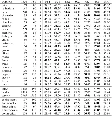
The F–measure associated with the discrimination of each word is shown in Table 1. Any score that is sig-nificantly greater than the majority sense (according to a paired t–test) is shown in bold face.

9

Analysis and Discussion

word.pos TRN TST S PB1 SC1 PB2 SC2 PB3 SC3 MAJ art.n 159 83 4 37.97 45.52 45.46 46.15 43.03 55.34 46.32 authority.n 168 90 4 38.15 51.25 43.93 53.01 41.86 34.94 37.76 bar.n 220 119 5 34.63 37.23 50.66 40.87 41.05 58.26 45.93 channel.n 135 67 6 40.63 37.21 40.31 41.54 36.51 39.06 31.88 child.n 116 62 2 45.04 46.85 51.32 50.00 55.17 53.45 56.45 church.n 123 60 2 57.14 49.09 48.21 55.36 52.73 46.43 59.02 circuit.n 129 75 8 25.17 34.72 32.17 33.33 27.97 25.35 30.26 day.n 239 128 3 60.48 46.15 55.65 45.76 62.65 55.65 62.94 facility.n 110 56 3 40.00 58.00 38.09 58.00 38.46 64.76 48.28 feeling.n 98 45 2 58.23 51.22 52.50 56.10 46.34 53.66 61.70 grip.n 94 49 5 45.66 43.01 58.06 53.76 49.46 49.46 46.67 material.n 111 65 5 32.79 40.98 41.32 47.54 32.79 47.54 42.25 mouth.n 106 55 4 54.90 47.53 60.78 43.14 43.14 47.06 46.97 post.n 135 72 5 32.36 37.96 48.17 30.88 30.88 32.36 32.05 blind.a 97 53 3 53.06 61.18 63.64 58.43 76.29 79.17 82.46 cool.a 102 51 5 35.42 39.58 38.71 34.78 33.68 38.71 42.86 fine.a 93 59 5 47.27 47.71 47.71 33.93 38.18 47.71 41.10 free.a 105 64 3 48.74 49.54 52.54 55.46 45.00 52.99 49.23 natural.a 142 75 4 34.72 35.21 33.56 30.99 32.40 38.03 35.80 simple.a 126 64 4 38.33 50.00 47.06 38.33 38.33 47.06 50.75 begin.v 507 255 3 59.36 40.46 40.40 43.66 70.12 42.55 64.31 leave.v 118 54 5 43.14 38.78 27.73 40.00 46.00 53.47 38.18 live.v 112 59 4 37.83 40.00 48.21 45.45 36.37 41.82 57.63 train.v 116 56 5 28.57 33.96 28.57 34.28 26.67 32.08 33.93

line.n 1615 1197 3 72.67 26.77 62.00 55.47 68.40 37.97 72.10 hard.a 2365 1592 2 86.75 67.42 41.18 73.22 87.06 63.41 87.44 serve.v 2365 1752 4 40.50 33.20 36.82 34.37 45.66 31.46 40.53 cool.a-train.v 197 102 8 22.34 39.00 25.25 40.61 22.57 41.00 22.86 fine.a-cool.a 185 104 7 27.86 42.36 33.83 47.72 35.00 42.05 24.79 fine.a-grip.n 177 99 7 36.84 49.48 33.50 45.02 31.41 49.48 24.19 leave.v-post.n 204 113 8 29.36 48.18 32.11 41.44 23.85 41.82 21.01 post.n-grip.n 208 117 8 28.44 43.67 28.44 41.05 26.55 34.21 20.90

Table 1: F-measures

where each contains around 4200 training and test in-stances combined. Mixed word are unique because they combined the instances of multiple target words and thereby have a larger number of senses to discriminate. Each type of data brings with it unique characteristics, and sheds light on different aspects of our experiments.

9.1 Senseval-2 data

Table 2 compares PB1 against PB3, and SC1 against SC3, when these methods are used to discriminate the 24 SENSEVAL-2 words. Our objective is to study the effect of using bigram features against co–occurrences in first (PB) and second (SC) order context vectors while using relatively small amounts of training data per word. Note that PB1 and SC1 use co–occurrence features, while PB3 and SC3 rely on bigram features.

This table shows the number of nouns (N), adjec-tives (A) and verbs (V) where bigrams were more effec-tive than co-occurrences (bigram>co-occur), less effec-tive (bigram<co-occur), and had no effect (bigram=co-occur).

Table 2 shows that there is no clear advantage to us-ing either bigrams or co–occurrence features in first or-der context vectors (PB). However, bigram features show clear improvement in the results of second order context vectors (SC).

N A V

7 1 2 bigram>co-occur PB 6 4 2 bigram<co-occur 1 1 0 bigram=co-occur 9 3 3 bigram>co-occur SC 4 1 1 bigram<co-occur 1 2 0 bigram=co-occur

Table 2: Bigrams vs. Co-occurrences

N A V

PB 9 4 1 rbr>upgma 4 0 2 rbr<upgma 1 2 1 rbr=upgma SC 8 1 3 rbr>upgma 2 5 0 rbr<upgma 4 0 1 rbr=upgma

Table 3: Repeated Bisections vs. UPGMA

However, second order context vectors indirectly rep-resent bigram features, and do not require an exact match between vectors in order to establish similarity. Thus, the poor performance of bigrams in the case of first or-der context vectors suggests that when dealing with small amounts of data, we need to boost or enrich our bigram feature set by using some other larger training source like a corpus drawn from the Web.

Table 3 shows the results of using the Repeated Bi-sections algorithm in vector space (PB) against that of using UPGMA method in similarity space. This ta-ble shows the number of Nouns, Adjectives and Verbs SENSEVAL-2 words that performed better (rbr>upgma), worse (rbr<upgma), and equal (rbr=upgma) when using Repeated Bisections clustering versus the UPGMA tech-nique, on first (PB) and second (SC) order vectors.

In short, Table 3 compares PB1 against PB2 and SC1 against SC2. From this, we observe that with both first order and second order context vectors Repeated Bisec-tions is more effective than UPGMA. This suggests that it is better suited to deal with very small amounts of sparse data.

Table 4 summarizes the overall performance of each of these experiments compared with the majority class. This table shows the number of words for which an experi-ment performed better than the the majority class, broken down by part of speech. Note that SC3 and SC1 are most often better than the majority class, followed closely by PB2 and SC2. This suggests that the second order con-text vectors (SC) have an advantage over the first order vectors for small training data as is found among the 24 SENSEVAL-2 words.

We believe that second order methods work better on

N A V TOTAL SC3>MAJ 8 3 1 12 SC1>MAJ 6 2 2 10 PB2>MAJ 7 2 0 9 SC2>MAJ 6 1 2 9 PB1>MAJ 4 1 1 6 PB3>MAJ 3 0 2 5

Table 4: All vs. Majority Class

smaller amounts of data, in that the feature spaces are quite small, and are not able to support the degree of ex-act matching of features between instances that first order vectors require. Second order context vectors succeed in such cases because they find indirect second order co– occurrences of feature words and hence describe the con-text more extensively than the first order representations. With smaller quantities of data, there is less possibil-ity of finding instances that use exactly the same set of words. Semantically related instances use words that are conceptually the same but perhaps not lexically. Sec-ond order context vectors are designed to identify such relationships, in that exact matching is not required, but rather words that occur in similar contexts will have sim-ilar vectors.

9.2 Line, Hard and Serve data

The comparatively good performance of PB1 and PB3 in the case of the Line, Hard and Serve data (see Table 1) suggests that first order context vectors when clustered with UPGMA perform relatively well on larger samples of data.

Moreover, among the SC experiments on this data, the performance of SC2 is relatively high. This further sug-gests that UPGMA performs much better than Repeated Bisections with larger amounts of training data.

These observations correspond with the hypothesis drawn from the SENSEVAL-2 results. That is, a large amount of training data will lead to a larger feature space and hence there is a greater chance of matching more fea-tures directly in the context of the test instances. Hence, the first order context vectors that rely on the immedi-ate context of the target word succeed as the contexts are more likely to use similar sets of words that in turn are selected from a large feature collection.

9.3 Mix-Word Results

words, which leads to a subset of coarse grained (distinct) senses within the data that are easier to discover than the senses of a single word.

Table 1 shows that the top 3 experiments for each of the mixed-words are all second order vectors (SC). We believe that this is due to the sparsity of the feature spaces of this data. Since there are so many different senses, the number of first order features that would be required to correctly discriminate them is very high, leading to better results for second order vectors.

10

Future Directions

We plan to conduct experiments that compare the ef-fect of using very large amounts of training data versus smaller amounts where each instance includes the tar-get word (as is the case in this paper). We will draw our large corpora from a variety of sources, including the British National Corpus, the English GigaWord Cor-pus, and the Web. Our motivation is that the larger cor-pora will provide more generic co–occurrence informa-tion about words without regard to a particular target word. However, the data specific to a given target word will capture the word usages in the immediate context of the target word. Thus, we will test the hypothesis that a smaller sample of data where each instance includes the target word is more effective for sense discrimination than a more general corpus of training data.

We are also planning to automatically attach descrip-tive labels to the discovered clusters that capture the un-derlying word sense. These labels will be created from the most characteristic features used by the instances be-longing to the same cluster. By comparing such descrip-tive features of each cluster with the words that occur in actual dictionary definitions of the target word, we plan to carry out fully automated word sense disambiguation that does not rely on any manually annotated text.

11

Conclusions

We present an extensive comparative analysis of word sense discrimination techniques using first order and sec-ond order context vectors, where both can be employed in similarity and vector space. We conclude that for larger amounts of homogeneous data such as the Line, Hard and

Serve data, the first order context vector representation

and the UPGMA clustering algorithm are the most effec-tive at word sense discrimination. We believe this is the case because in a large sample of data, it is very likely that the features that occur in the training data will also occur in the test data, making it possible to represent test in-stances with fairly rich feature sets. When given smaller amounts of data like SENSEVAL-2, second order context vectors and a hybrid clustering method like Repeated Bi-sections perform better. This occurs because in small and

sparse data, direct first order features are seldom observed in both the training and the test data. However, the in-direct second order co–occurrence relationships that are captured by these methods provide sufficient information for discrimination to proceed.

12

Acknowledgments

This research is supported by a National Science Foun-dation Faculty Early CAREER Development Award (#0092784).

All of the experiments in this paper were carried out with version 0.47 of the SenseClusters package, freely available from the URL shown on the title page.

References

S. Deerwester, S.T. Dumais, G.W. Furnas, T.K. Landauer, and R. Harshman. 1990. Indexing by latent semantic analysis. Journal of the American Society for

Informa-tion Science, 41:391–407.

F. Fukumoto and Y. Suzuki. 1999. Word sense disam-biguation in untagged text based on term weight learn-ing. In Proceedings of the Ninth Conference of the

Eu-ropean Chapter of the Association for Computational Linguistics, pages 209–216, Bergen.

T.K. Landauer, P.W. Foltz, and D. Laham. 1998. An in-troduction to latent semantic analysis. Discourse

Pro-cesses, 25:259–284.

G.A. Miller and W.G. Charles. 1991. Contextual corre-lates of semantic similarity. Language and Cognitive

Processes, 6(1):1–28.

T. Pedersen and R. Bruce. 1997. Distinguishing word senses in untagged text. In Proceedings of the

Sec-ond Conference on Empirical Methods in Natural Lan-guage Processing, pages 197–207, Providence, RI,

August.

T. Pedersen and R. Bruce. 1998. Knowledge lean word sense disambiguation. In Proceedings of the Fifteenth

National Conference on Artificial Intelligence, pages

800–805, Madison, WI, July.

A. Purandare. 2003. Discriminating among word senses using McQuitty’s similarity analysis. In Proceedings

of the HLT-NAACL 2003 Student Research Workshop,

pages 19–24, Edmonton, Alberta, Canada, May.

H. Sch¨utze. 1992. Dimensions of meaning. In

Pro-ceedings of Supercomputing ’92, pages 787–796,

Min-neapolis, MN.

H. Sch¨utze. 1998. Automatic word sense discrimination.

Computational Linguistics, 24(1):97–123.

Y. Zhao and G. Karypis. 2002. Evaluation of hierar-chical clustering algorithms for document datasets. In