Latent Ambiguity in Latent Semantic Analysis?
Martin Emms and Alfredo Maldonado-Guerra
School of Computer Science and Statistics, Trinity College, Dublin, Ireland {mtemms,maldonaa}@tcd.ie
Keywords: LSA; Dimensionality
Abstract: Latent Semantic Analyis (LSA) consists in the use of SVD-based dimensionality-reduction to reduce the high dimensionality of vector representations of documents, where the dimensions of the vectors correspond simply to word counts in the documents. We show that that there are two contending, inequivalent, formulations of LSA. The distinction between the two is not generally noted and while some work adheres to one formulation, other work adheres to the other formulation. We show that on both a tiny contrived data-set and also on a more substantial word-sense discovery data-set that the empirical outcomes achieved with LSA vary according to which formulation is chosen.
1
Introduction
Latent Semantic Analyis (LSA) is a widely used dimensionality-reduction technique. Section 2 re-calls the matrix properities upon which LSA is based and then section 3 gives details of two different dimensionality-lowering transformations which may be based on those properites, which we will term the R1and R2representations, and we argue that there is ambiguity in the literature as to which representation is intended. Section 4 then shows empirical outcomes which vary with the adopted formulation.
2
Singular Value Decomposition
Latent Semantic Analysis (LSA) is based theoret-ically and algorithmtheoret-ically on Singular Value Decom-position (SVD) properties of matrices. The first con-cerns the existence of a particular decomposition, a property expressible as the following theorem1 Theorem 1 (SVD). if m×n matrix A has rank r, then it can be factorised as A=USV′where:
1. U has the eigen-vectors of A×A′ for its first r columns, in descending eigen-value order; these columns are orthonormal
2. S has zeroes everywhere, except its diagonal which has the square roots of the r distinct eigen-values of U, in descending order, then 0
1This follows closely Theorem 18.3 of (Manning et al.,
2008)
3. V has the eigen-vectors of A′×A for its first columns, in descending eigen-value order; these column are orthonormal
Without loss of generality once can assume the di-mensions of the matrices are:
U : m×r,S : r×r,V : n×r
The second essential fact is that the SVD can be used to derive optimum2low-rank approximations of the orginal A, by truncating the SVD of A to use just the first k columns of U and V as follows (see again (Manning et al., 2008))
Theorem 2 (Low rank approximation). If U×S×V′ is the SVD of A, then ˆA=Uk×Sk×V′kis a optimum rank-k approx of A where
1. Skis diagonal with top-most k values from S 2. Ukis just first k columns of U
3. Vkis just first k columns of V
Uk×Sk×V′kcan be termed the ’rank k reduced SVD
of A’.
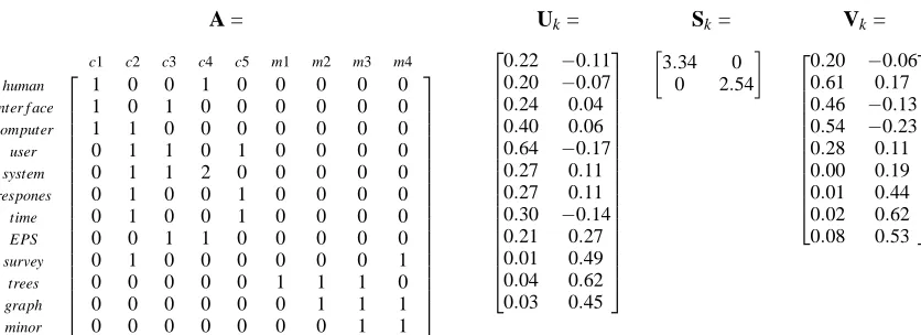
The HCI/Graph Example Figure 1 shows a 12×9 term-by-document matrix, A (ie. rows of A express terms via their document occurrence, columns of A express documents via their term occurrence). This term-by-document matrix is used in a number of arti-cles by the originators of LSA. See (Deerwester et al.,
2Optimality being defined as minimising the sum of
A = Uk= Sk= Vk=
c1 c2 c3 c4 c5 m1 m2 m3 m4
human 1 0 0 1 0 0 0 0 0
inter f ace 1 0 1 0 0 0 0 0 0
computer 1 1 0 0 0 0 0 0 0
user 0 1 1 0 1 0 0 0 0
system 0 1 1 2 0 0 0 0 0
respones 0 1 0 0 1 0 0 0 0
time 0 1 0 0 1 0 0 0 0
EPS 0 0 1 1 0 0 0 0 0
survey 0 1 0 0 0 0 0 0 1
trees 0 0 0 0 0 1 1 1 0
graph 0 0 0 0 0 0 1 1 1
minor 0 0 0 0 0 0 0 1 1
0.22 −0.11 0.20 −0.07 0.24 0.04 0.40 0.06 0.64 −0.17 0.27 0.11 0.27 0.11 0.30 −0.14 0.21 0.27 0.01 0.49 0.04 0.62 0.03 0.45 3.34 0 0 2.54
0.20 −0.06 0.61 0.17 0.46 −0.13 0.54 −0.23 0.28 0.11 0.00 0.19 0.01 0.44 0.02 0.62 0.08 0.53
Figure 1: A term-by-document matrix A, and the components matrices of its rank 2 reduced SVD UkSkV′k
1990; Landauer et al., 1998). It is based on an artifi-cial data set concerning two sets of article titles, one about HCI (titles c1–c5), the other about graph theory (titles m1–m4). The columns count occurrences of 12 chosen terms. This A has rank 9, and has a SVD de-composition into U×S×V′, where U is 12×9, and V is 9×9 . See p406 of (Deerwester et al., 1990).
Multiplying U, S and V′gives back exactly A. To the right in Figure 1 the component matrices Uk, Sk,
Vkof its rank 2 reduced SVD are given, whereby ˆA=
UkSkV′k(see also p406 of (Deerwester et al., 1990)).
3
Contending formulations of LSA
LSA concerns using the SVD to make lower di-mension versions of the columns of A (or vectors like these ie. m dimensional ’document’ vectors).
Where d is an m dimensional vector (such as a column of A), we contend that the literature has ba-sically two contenders for its SVD-based reduced di-mensionality version, contenders we shall term R1(d) and R2(d).
Definition 1 (R1and R2document projections). If A is m×n, and UkSkV′kis its rank k reduced SVD, and
d is an m dimensional vector, then k-dimensional ver-sions R1(d)and R2(d)are defined by
R1(d) = d×Uk (1)
R2(d) = d×Uk×Sk−1=R1(d)×S−k1 (2) and if d is ith column of A and Vik is ith row of Vk (ie.[V(i,1). . .V(i,k)]) the above defintions are equiv-alent to
R1(d) = Vik×Sk (3)
R2(d) = Vik (4)
That the alternative formulations in (3) and (4) are equivalent to the formulations in (1) and (2), for the case where d is a column of A, is not immediately apparent. You can show the equivalence of (3) and (1), that is, d×Uk=Vik×S when d is the ithcolumn
of A starting from the defining SVD equation A=
USV′as follows:
A′ = (USV′)′ = VSU′
hence A′U = VSU′U = VS hence dUk = VkSk
The equivalence of (4) and (2), that is, d×Uk×S−1=
Vik when d is the ith column of A, follows from the equivalence of (3) and (1) by post-multiplication by S−1
Where A is a m×n matrix, the matrix Vkof its
re-duced SVD is a n×k matrix. For the example shown in Figure 1, Vkhas exactly as many rows (9) as there
were column vectors representing documents in the original term-by-document matrix A. Therein lies the possibility to identify these rows of Vkas the reduced
representation of the columns of A. The fact that (2) is equivalent to (4) leads to the naturally accompanying assumption that (2) – d×Uk×S−1– is the formula
for projecting an arbitrary document vector d. On the other hand, where A is a m×n matrix, the matrix Uk of its reduced SVD is a m×k matrix, so
[image:2.595.85.503.91.243.2]its columns are of exactly the size for it to be possible to take dot products with an m dimensional document vector, as expressed in (1). For the example shown in Figure 1 the columns of the matrix Ukof A’s reduced
SVD are of size 12, the same as that of document vec-tors. Additionally the columns of Uk are orthogonal
to each other and of unit length and thus the R1 for-mulation is simply the projection onto a new set of orthogonal axes defined by the columns of Uk.
R1(d)×S−1. However, since the entries on the diag-onal of S are not equal, such a scaling changes the es-sential geometry. In particular, the nearest neighours, or the set within a certain cosine range of a given vec-tor d, is not generally preserved under a scaling. For example, given a scaling which transforms x and y according to x′=x
2, y′= y
8, the table below gives the coordinates of 3 points before and after the scaling:
a (0,8) a′ (0,1) b (4,8) b′ (2,1) c (4,0) c′ (2,0)
and before the scaling b has nearest neighbour a, whilst afterwards b′has nearest neighbour c′, on both the euclidean distance and cosine measures. Machine learning methods for adapting distance measures are often predicated on precisely this fact. In view of this, the R1formulation of LSA, as expressed by (1) and (3) is genuinely different to the R2formulation, as ex-pressed by (2) and (4) and one should expect R1and R2to give diverging outcomes when deployed within a system. We contend that this has been overlooked. To this end we will consider the work of a number of authors, arguing that some are adhering to the R1 formulation and some to the R2formulation.
The R2 formulation of LSA is one presented in many, fairly widely cited, publications, for example (Rosario, 2000; Gong and Liu, 2001; Zelikovitz and Hirsh, 2001), the relevant parts of which are below briefly noted.
In the notation of (Rosario, 2000), the reduced rank SVD of the t×d, term-by-document matrix is Tt×kSk×k(Dd×k)T, with T and D used in place of Uk
and Vk. This is described (p3) as providing a
repre-sentation in an alternative space whereby the matrices T and D represent terms and doc-uments in this new space
and additionally the repesentation of a query is given (p4) as qTTt×kS−k×1k. Thus for pre-existing documents
and novel queries, this matches, modulo notational switches, the R2formulations of (4) and (2).
In the notation of (Zelikovitz and Hirsh, 2001), the SVD of a t×d term-by-document matrix is T SDT. The representation of a query, based on this SVD is given as
a query is represented in the same new small space that the document collection is repre-sented in. This is done by multiplying the transpose of the term vector of the query with matrices T and S−1
Again modulo notational switches, this is the R2 for-mulation of (2).
In the notation of (Gong and Liu, 2001), the SVD of an m×n term-by-sentence matrix is UΣVT, and the SVD is described as defining a mapping which (p21)
projects each column vector i in matrix A . . . to column vector Φi = [vi1vi2. . .vir]
T of
matrix VT
thus the i-th column of A is represented by the i-th row of V, which is the R2formulation given in (4).
On the other hand, the R1formulation of LSA is also presented in many, fairly widely cited, publica-tions, for example (Bartell et al., 1992; Papadimitriou et al., 2000; Kontostathis and Pottenger, 2006), the relevant parts of which are below briefly noted.
In the notation of (Bartell et al., 1992) the reduced rank SVD of a term-by-document matrix is UkLkATk,
and their definitions of document and query represen-tations are (p162)
row i of AkLkgives the representation of doc-ument i in k-space. . . . Let the query be en-coded as a row vector q in
R
t. Then the query in k-space would be qUkThese coincide, modulo notational differences, with the R1formulations of (3) and (1).
In the notation of (Papadimitriou et al., 2000) the reduced rank SVD of a term-by-document matrix is UkDkVkT. Then concerning document representation
they have (p220)
The rows of VkDkabove are then used to rep-resent the documents. In other words, the col-umn vectors of A (documents) are projected to the k-dimensional space spanned by the col-umn vectors of Uk
which coincides, modulo notation, with the R1 formu-lations in (3) and (1).
In the notation of (Kontostathis and Pottenger, 2006), the reduced rank SVD of a term-by-document matrix is TkSk(Dk)T, with Tkand Dkused in place of
Uk and Vk. Their definition of query representation
and document representation is (p3)
Queries are represented in the reduced space by TkTq. . . . Queries are compared to the re-duced document vectors, scaled by the singu-lar values (SkDTk)
These column vector formulations would be a row vector formulation qTkand DkSk, which, modulo
no-tational differences are the R1formulations of (1) and (3).
−0.5 0.0 0.5 1.0 1.5 2.0 2.5
−1.0
−0.5
0.0
0.5
1.0
1.5
2.0
c1
c2
c3
c4 c5
m1 m2
m3
m4
[image:4.595.88.492.99.293.2]q1 q2
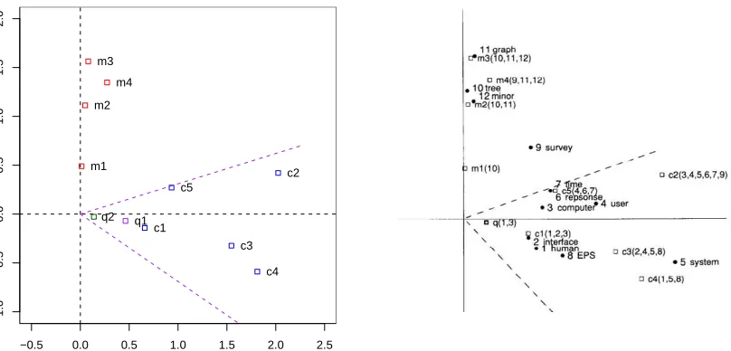
Figure 2: Left: shows the R1representation of the c1–c5 and m1–m4 documents from Figure 1 and as q1 and q2, the R1and
R2representations of the query from the text; also shows cosine 0.9 cone around q1 Right screen shot from (Deerwester et al.,
1990), also showing c1–c5, m1–m4 and the query
et al., 1990). We shall see that there is ambiguity as to whether it is the R1or R2representation that is in-tended by the text of (Deerwester et al., 1990).
Recall that Figure 1 showed the basic term-by-document matrix for this example, and the component matrices of its rank-2 reduced SVD. The two dimen-sional nature of the reduced representations allows for simple plotting. The left part of Figure 2 plots the 9 documents using the R1projection, based on the rank-2 reduced SVD shown in Figure 1. The positions of the documents are indicated by boxes labelled ’c’ and ’m’.
To the right in Figure 2 is a reproduction of the figure on p397 of (Deerwester et al., 1990). Their plot shows (amongst other things) a reduced repre-sentation of the documents, as boxes labeled c1-c5 and m1-m4. Whether their plot is intended to depict the documents in the R1or R2representation is moot: the axes in the original plot are not labeled. We have endeavoured to scale the two plots in such a way that the document vectors are identically placed in the two pictures.
In (Deerwester et al., 1990), they consider the query ’human computer interaction’. Given the terms chosen for the document vectors, the unreduced vec-tor q is [1,0,1,0,0,0,0,0,0,0,0,0]. Applying the R1 definition (1), we have R1(q) = [0.46,−0.07] and applying the R2 definition (2), we R2(q) = [0.14,−0.03]. We have plotted these alternative re-ductions of q also in the left part of Figure 2, where they are are shown as q1 and q2.
In the plot reproduced from (Deerwester et al.,
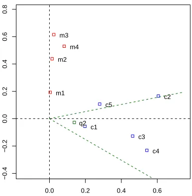
1990) a reduced image of the same query vector was depicted. Considering their placement of the repre-sentation of the query relative to the document rep-resentations, and comparing it to our own placment of its R1and R2representation relative to the R1 rep-resentations of the documents, it seems the only in-terpretation that can be put on the plot from (Deer-wester et al., 1990) is that it shows the documents in the R1projection, but the query in the the R2 projec-tion. Note that because the R2representation is sim-ply a scaling of the R1representation, with a different scaling of each dimension, the relative position of the document and query points in the plot from (Deer-wester et al., 1990) is not consistent with all points being shown in the R2representation. To emphasize this, Figure 3 gives the plot of documents and query in the R2representation, again in such a way that the documents are positioned identically to the plot from (Deerwester et al., 1990) and one can see that the query representations are differently placed.
This seeming equivocation between the R1and R2 projection occurs in the text of (Deerwester et al., 1990) also. In their notation the SVD of the term-by-document matrix is T SD′, thus using T and D in place of our U and V. Concerning document representation, there is (p398)
’the rows of the reduced matrices of singular vectors are taken as coordinates of points rep-resenting the documents and terms in a k di-mensional space’
As we noted above, identifying the rows of Vkas the
adopt-ing the R2 representation (see (4)). Concerning a query, if its unreduced representation as a column vector is Xq, they give its reduced representation as Xq′T S−1, which again, modulo notation, is the R2 for-mulation (see (2))
On the other hand p399 has (recall their ’D’ is Vk
in our notation)
so one can consider rows of a DS matrix as coordinates for documents, and take dot prod-ucts in this space . . . note that the DS space is just a stretched version of the D space
As we noted above, in equation (3), this amounts to adopting the R1representation for documents.
4
Contrasting outcomes
Setting aside these expository details, it is more important to know whether system outcomes may change according to which representation, R1or R2, is adopted. The LSA dimensionality reduction tech-nique has been deployed in quite a variety of con-texts and in each one might investigate the effect of whether R1or R2is adopted. In this section we con-sider two such contexts.
The first context is the original one presented in (Deerwester et al., 1990): the issue is which docu-ments should count as similar to a given query un-der the two representations. Returning again to the HCI/Graph example, in our R1depiction of the docu-ments and query that is the left-hand plot of Figure 2, we have also shown a cone which encloses the points that have a cosine value of 0.9 or higher to R1(q). Fig-ure 3 shows the documents and the query q instead in the R2projection, and shows the corresponding cone around R2(q).
On the R1 projection, the representations of c1– c5 are all included in the cone around the query. In (Deerwester et al., 1990), this inclusion of all the HCI document representations (c1–c5) within cosine 0.9 of the given query is also noted, notwithstanding the above-noted R1-vs-R2 ambiguities concerning their plot of the data. As Figure 3 shows, on the R2 projec-tion (of queries and documents), the representaprojec-tions of c5 and c2 are not included. Note that the visual similarity of Figure 3 and the left part of Figure 2 is a bit misleading, as the values on the axes in the R2 rep-resentation in Figure 3 are considerably smaller than those on the axes in the R1representation, (by a fac-tor of 0.29 for the first dimension, and 0.39 for the second).
Another context in which LSA dimensionality re-duction has been used is in word clustering. The aim
0.0 0.2 0.4 0.6
−0.4
−0.2
0.0
0.2
0.4
0.6
0.8
c1
c2
c3
c4 c5
m1 m2
m3
m4
[image:5.595.312.505.90.287.2]q2
Figure 3: The R2representation of the c1–c5 and m1–m4
documents from Figure 1 and as q2 the R2representation of
the query from the text; also shows cosine 0.9 cone around q2
is to cluster occurrences of an ambiguous word into coherent clusters, clusters each of which reflect a dis-tinct sense of the word. To this end each occurrence of an ambiguous term at a position p is represented by its so-called first-order context vector, C1(p), a vec-tor which for a given uni-gram vocabularyΣf records
for each unigram its frequency in the window between p−10 and p+10.
We conducted an experiment making use of the so-called HILS dataset, which consists of manually sense annotated occurrences of the four words hard-interest-line-serve. Thus for each word there is a sub-corpus consisting of its occurrences, and for each word, a 60% subset was taken and clustered by the k-means algorithm, where k is set to the number of attested senses of the given word. The clustering is evaluated using the remaining 40% test-set: these items are first assigned to their nearest cluster centres and then for each possible sense-to-cluster mapping, a precision score on the test set is determined, with the maximum of these reported as the final score.
2 4 6 8 10 12 14
20
30
40
50
60 R1
R2 hard
2 4 6 8 10 12 14
20
30
40
50
60 R1
R2 interest
2 4 6 8 10 12 14
20
30
40
50
60 R1
R2 line
2 4 6 8 10 12 14
20
30
40
50
60 R1
[image:6.595.76.279.92.294.2]R2 serve
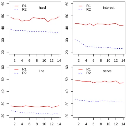
Figure 4: Unsupervised clustering results using R1and R2
representations. Vertical axis is accuracy, horizontal axis is % reduction of dimensions.
for the various words the 10% reduction level corre-sponds to a dimensionality of 856(hard), 494(inter-est), 1297(line) and 1304(serve). From these reduced SVDs, the thereby defined R1and R2versions of the context vectors were then used. Figure 4 gives the results (the 60-40 split was randomly made, and re-peated 4 times, with the figure summarising the out-comes over these splits).
This confirms the indications from the tiny 2-dimensional HCI/Graph example, namely that the outcomes under the R1and R2representations are not identical. In this word clustering context, at each level of reduction, the outcomes with the R1and R2 repre-sentations are clearly different. In fact there is a per-sistent pattern of the R1representation giving consis-tently better outcomes than the R2representation.
5
Conclusion
We have shown that there is a discrepancy amongst researchers concerning the precise dimen-sionality reduction technique to which they give the name ’LSA’. The R1 representation is defined by equations (1) and (3) whilst the R2representation is defined by (2) and (4), and these alternatives give a different geometry to the space of reduced representa-tions, manifesting itself in different nearest-neighbour sets. We showed that, unsurprisingly, this can lead to different system outcomes according to which repre-sentation, R1or R2, is adopted in a given system.
We have not argued for one of these
representa-tions over the other one. Whilst Theorem 2 estab-lishes that ˆA=Uk×Sk×V′k is the optimum rank-k
approximation of A in the sense of minimising the sum of squared differences between corresponding matrix positions, there is a good deal of conceptual clear water between this and consequent ’optimality’ of a particular SVD-based reduction of document vec-tors in a particular system. This is testified to by the range of attempts there have been to give a theoretical justification for an observed system ’optimality’ of a given deployed SVD-based reduction. Therefore the R1and R2alternatives are as theoretically motivated (or unmotivated) as each other, at least at first glance, and there is some merit in putting both to the test em-pirically. What is beyond doubt, though, is that these R1and R2altneratives are genuinely different and will not always give the same empirical outcomes.
Acknowledgements
This research is supported by the Science Founda-tion Ireland (Grant 07/CE/I1142) as part of the Cen-tre for Next Generation Localisation (www.cngl.ie) at Trinity College Dublin.
REFERENCES
Bartell, B. T., Cottrell, G. W., and Belew, R. K. (1992). Latent semantic indexing is an optimal special case of multidimensional scaling. In Proceedings of the Fifteenth Annual International ACM SIGIR Confer-ence on Research and Development in Information Retrieval, pages 161–167. ACM Press.
Deerwester, S., Dumais, S. T., Furnas, G. W., Landauer, T. K., and Harshman, R. (1990). Indexing by latent se-mantic analysis. JOURNAL OF THE AMERICAN SO-CIETY FOR INFORMATION SCIENCE, 41(6):391– 407.
Gong, Y. and Liu, X. (2001). Generic text summarization using relevance measure and latent semantic analysis. In SIGIR, pages 19–25.
Kontostathis, A. and Pottenger, W. M. (2006). A frame-work for understanding latent semantic indexing (lsi) performance. INFORMATION PROCESSING AND MANAGEMENT, 42(1):56–73.
Landauer, T., Foltz, P., and Laham, D. (1998). An introduc-tion to latent semantic analysis. Discourse Processes, 25(1):259–284.
Manning, C. D., Raghavan, P., and Sch¨utze, H. (2008). In-troduction to Information Retrieval. Cambridge Uni-versity Press.
Rosario, B. (2000). Latent semantic indexing: An overview. Technical report, Berkeley University. available at http://people.ischool.berkeley. edu/˜rosario/projects/LSI.pdf.