An Improved Switching Hybrid Recommender
System Using Naive Bayes Classifier and
Collaborative Filtering
Mustansar Ali Ghazanfar and Adam Pr¨
ugel-Bennett
∗Abstract— Recommender Systems apply machine learning and data mining techniques for filtering un-seen information and can predict whether a user would like a given resource. To date a number of rec-ommendation algorithms have been proposed, where collaborative filtering and content-based filtering are the two most famous and adopted recommendation techniques. Collaborative filtering recommender sys-tems recommend isys-tems by identifying other users with similar taste and use their opinions for recom-mendation; whereas content-based recommender sys-tems recommend isys-tems based on the content informa-tion of the items. These systems suffer from scalabil-ity, data sparsscalabil-ity, over specialization, and cold-start problems resulting in poor quality recommendations and reduced coverage. Hybrid recommender systems combine individual systems to avoid certain afore-mentioned limitations of these systems. In this paper, we proposed a unique switching hybrid recommenda-tion approach by combining a Naive Bayes classifica-tion approach with the collaborative filtering. Exper-imental results on two different data sets, show that the proposed algorithm is scalable and provide better performance–in terms of accuracy and coverage–than other algorithms while at the same time eliminates some recorded problems with the recommender sys-tems.
Keywords: Hybrid Recommender Systems; Collabora-tive Filtering; Content-Based Filtering; Naive Bayes Classifier.
1
Introduction
There has been an exponential increase in the volume of available digital information, electronic sources, and on-line services in recent years. This information overload has created a potential problem, which is how to filter and efficiently deliver relevant information to a user. Further-more, information needs to be prioritized for a user rather than just filtering the right information, which can create information overload problems. Search engines help in-ternet users by filtering pages to match explicit queries, but it is very difficult to specify what a user wants by
∗School of Electronics and Computer Science, University of
Southampton, Highfield Campus, SO17 1BJ, United Kingdom. Email: {mag208r, adp}@ecs.soton.ac.uk
using simple keywords. The Semantic Web, also provides some help to find useful information by allowing intelli-gent search queries, however it depends on the extent the web pages are annotated.
These problems highlight a need for information extrac-tion systems that can filter unseen informaextrac-tion and can predict whether a user would like a given source. Such systems are called recommender systems, and they mit-igate the aforementioned problems to a great extent. Given a new item, recommender systems can predict with impressive accuracy whether a user would like this item or not, based on user preferences (likes- positive examples, and dislikes- negative examples), observed behaviour, and information (demographic or content information) about items [1, 2].
An example of the recommender system is the Amazon1
recommender engine [3], which can filter through millions of available items based on the preferences or past brows-ing behaviour of a user and can make personal recommen-dations. Some other well-known examples are Youtube2
video recommender service and MovieLens3
movie rec-ommender system, which recommend videos and movies based on the person’s opinions. In these systems, a his-tory of user’s interactions with the system is stored which given rise to his preferences. The history of the user can be gathered by explicit feedback, where the user rates some items in some scale or by implicit feedback, the user’s interaction with the item is observed- for instance, if a user purchases an item then this is a sign that he likes that item, his browsing behaviour, etc.
There are two main types of recommender systems: col-laborative filtering and content-based filtering recom-mender systems. Collaborative filtering recommender systems [4, 5, 6, 7] recommend items by taking into ac-count the taste (in terms of preferences of items) of users, under the assumption that users will be interested in items that users similar to them have rated highly. Ex-amples of these systems include GroupLens system [8],
1
www.amazon.com 2
www.youtube.com 3
Ringo4
, etc. Collaborative filtering classified into two sub-categories: memory-based CF and model-based CF. Memory-based approaches [5] make a prediction by tak-ing into account the entire collection of previous rated items by a user, examples include GroupLens recom-mender systems [8]. Model-based approaches [9] use rat-ing patterns of users in the trainrat-ing set, group users into different classes, and use ratings of predefined classes to generate recommendation for an active user5
on a tar-get item6
, examples include item-based CF [10], Singular Value Decomposition (SVD) based models [11], bayesian networks [12], and clustering methods [13].
Content-based filtering recommender systems [14] recom-mend items based on the textual information of an item, under the assumption that users will like similar items to the ones they liked before. In these systems, an item of interest is defined by its associated features, for in-stance, NewsWeeder [15], a newsgroup filtering system uses the words of text as features. The textual descrip-tion of items is used to build item profiles. User profiles can be constructed by building a model of the users pref-erences using the descriptions and types of the items that a user is interested in, or a history of users interactions with the system is stored (e.g. user purchase history, types of items he purchases together, his ratings, etc.). The history of the user can be gathered by explicit feed-back or implicit feedfeed-back. Explicit feedfeed-back is noise free but the user is unlikely to rate many items, whereas, im-plicit feedback is noisy (error prone), but can collect a lot of training data [16]. In general, a trade-off between implicit and explicit user feedback is used. Creating and learning user profiles is a form of classification problem, where training data can be divided into two categories: items liked by a user, and item disliked by a user.
Recommendations can be presented to an active user in the followings two different ways: by predicting ratings of items a user has not seen before and by constructing a list of items ordered by his preferences. In the former case, an active user provides the prediction engine with the list of items to be predicted, prediction engine uses other users (or items) ratings or content information, and then predict how much the user would like the given item in some numeric or binary scale. In the latter case, different heuristics are used for producing an ordered list of items, sometimes termed as top-N recommendations [11, 17]. For example, in collaborative filtering recommender sys-tem this list is produced by making the rating predictions of all items an active user has not yet rated, sorting the list, and then keeping the top-N items the active user would like the most. In this paper, we focussed on the former case–predicting the ratings of items–however we can easily construct a list of top-N items for each user by
4
www.ringo.com 5
The user for whom the recommendations are computed. 6
The item a system wants to recommend.
selecting highly predicted items.
1.1
Problem Statement
The continuous increase of the users and items demands the following properties in a recommender system. First is thescalability, that is its ability to generate predictions quickly in user-item rating matrix consisting of millions of users and items. Second is to find good items and to ameliorate the quality of the recommendation for a cus-tomer. If a customer trusts and leverages a recommender system, and then discovers that he is unable to find what he wants then it is unlikely that he will continue with that system. Consequently, the most important task for a recommender system is to accurately predict the rating of the non-rated user/item combination and recommend items based on these predictions. These two properties are in conflict, since the less time an algorithm spends searching for neighbours, the more scalable it will be, but produces worse quality recommendations. Third its coverage should be maximum, i.e. it should be able to produce recommendation for all the existing items and users regardless of thenew item cold-start7
andnew user cold-start8
problems. Fourth, its performance should not degrade withsparsity. As the user-item rating matrix is very sparse, hence the system may be unable to make many product recommendation for a particular user.
Collaborative Filtering and Content-based filtering suf-fer from potential problems– such as over-specialization9
, sparsity, reduced coverage, scalability, and cold-start problems, which reduce the effectiveness of these sys-tems. Hybrid recommender systems have been proposed to overcome some of the aforementioned problems. In this paper, we propose a switching hybrid recommender system [18] using naive Bayes and item-based CF. A switching hybrid system is intelligent in a sense that it can switch between recommendation techniques using some criterion. The benefit of switching hybrid is that it can make efficient use of strengths and weaknesses of its constitutional recommender systems. We show em-pirically that proposed recommender system outperform other recommender system algorithms in terms of MAE, ROC-Sensitivity, and coverage. We evaluate our
algo-7
When a new item is added to the system, then it is not possible to get rating for that item from significant number of users, and consequently the CF recommender system would not be able to recommend that item. This problem is called new itemcold-start problem [9].
8
CF recommender system works by finding the similar users based on their ratings, however it is not possible to get ratings from a newly registered user. Therefore, the system cannot recom-mend any item to that user, a potential problem with recomrecom-mender system callednew user cold-start problem [9].
9
rithm on MovieLens10
and FilmTrust11
datasets.
The rest of the paper has been organized as follows. Sec-tion 2 discusses the related work. SecSec-tion 3 presents some background concepts relating to item-based CF, content-based filtering, and Naive Bayes classifier. Section 4 out-lines the proposed algorithm. Section 5 describes the data set and metrics used in this work. Section 6 compares the performance of the proposed algorithm with the existing algorithms followed by conclusion in section 7.
2
Related Work
Pazzani [19] propose a hybrid recommendation approach in which a content-based profile of each user is used to find the similar users, which are used for making pre-dictions. The author used Winnow to extract features from user’s home page to build the user content-based profile. The problem with this approach is that if the content-based profile of a user is erroneous (may be due to synonyms problems or others), then it will results in poor recommendations. In [20], the authors proposed a hybrid recommender framework to recommend movies to users. In the content-based filtering part, they get extra information about movies from the IMDB12
web site and view each movie as a text document. A Naive Bayes clas-sifier is used for building user and item profiles, which can handle vectors of bags-of-words. The Naive Bayes clas-sifier is used to approximate the missing entries in the user-item rating matrix, and a user-based CF is applied over this dense matrix. The problem with this approach is that it is not scalable. Our work combines Naive Bayes and Collaborative Filtering in a more scalable way than [20] and uses synonym detection and feature selection al-gorithms that produce accurate profiles of users resulting in improved predictions. The off-line cost of our approach and [20] is the same, i.e. the cost to build a naive Bayes classifier. However, our on-line cost (in the worse case) is less than or equal to [20]13
. A similar approach has been used in a book recommender system, LIBRA [21]. LI-BRA downloads content information about book (meta data) from Amazon and extracts features using simple pattern-based information extraction system, and builds user models using a Naive Bayes classifier. A user can rate items using a numeric scale from 1 (lowest) to 10 (highest). It does not predict exact values, but rather presents items to a user according to his preferences. The authors in [22, 23] used demographic information about users and items for providing more accurate prediction for user-based and item-based CF. They proposed hy-brid recommender system (lying between cascading and feature combination hybrid recommender systems [18]) in which demographic correlation between two items (or
10
www.grouplens.org/node/73 11
www.filmtrust.com 12
www.imdb.com 13
See section 6.
users) is applied over the candidate neighbours found af-ter applying the rating correlation on the user-item rat-ing matrix. This refined set of neighbours are used for generating predictions. However they completely miss the features of items for computing similarity. In [24], content-based filtering using the Rocchio’s method is ap-plied to maintain a term vector model that describe the user’s area of interest. This model is then used by collab-orative filtering to gather documents on basis of interest of community as a whole. Another example of hybrid systems is proposed in [25], where the author presented an on-line hybrid recommender system for news recom-mendation.
3
Background
LetM ={m1, m2,· · ·, mx}be the set of all users,N =
{n1, n2,· · ·, ny }be the set of all possible items that can
be recommended, andrmi,nj be the rating of usermion
itemnj.
3.1
Item-Based Collaborative Filtering
Item-based CF [10] builds a model of item similarities us-ing an off-line stage. Suppose we want to make prediction for an item nt for an active userma. LetMninj be the
set of all users, who have co-rated itemniandnj. There
are three main steps in this approach as follows:
• In the first step, all items rated by an active user are retrieved.
• In the second step, target item’s similarity is com-puted with the set of retrieved items. A set of K most similar items n1, n2· · ·nK with their
similarities sn1, sn2· · ·snK are selected. Similarity
sim(ni, nj), between two items ni and nj, is
com-puted by first isolating the users who have rated these items (i.e. Mninj), and then applying the
Ad-justed Cosine similarity [10] as follows:
sim(ni, nj) =
X
m∈Mni,nj
ˆ
rm,niˆrm,nj
s X
m∈Mni,nj
(ˆrm,ni)
2 X
m∈Mni,nj
(ˆrm,nj)
2
.
(1)
Where, ˆrm,n=rm,n−rm, i.e. normalizing a rating
by subtracting the respective user average from the rating, which is helpful in overcoming the discrepan-cies in user’s rating scale. We multiplied similarity weights with aSignificance Weigthing factor [26].
weighted sum, the prediction pma,nt on itemnt for
userma is computed as follows:
Pma,nt =
K
X
i=1
(snt,i×rma,i)
K
X
i=1
(|snt,i|)
. (2)
3.2
Content-Based Filtering:
Feature
Ex-traction and Selection
Feature extraction techniques aim at finding the specific pieces of data in natural language documents [27], which are used for building both users and items profiles. These users and items profiles are then employed by a classifier for recommending resources. Documents, which typically are strings of characters, are transformed into a represen-tation suitable for machine learning algorithms [28]. The documents are first converted into tokens, sequence of letters and digits, and then after stop word14
removal, stemming15
is performed . Each document is usually represented by a vector of n weighted index terms. A Vector Space Model [16] is the most commonly used doc-ument representation technique, in which docdoc-uments are represented by vectors of words. Term Frequency-Inverse Document Frequency (TF-IDF) approach or others [28] can be used for determining the weight of a word in a document. TF-IDF approach is a well-known approach and uses the frequency of a word in a document as well as in the collection of documents for computing weights.
The feature space in a typical vector space model can be very large, which can be reduced by feature selection pro-cess. Feature selection process reduces the feature space by eliminating useless noise words having little (or no) discriminating power in a classifier, or having low signal-to-noise ratio. Several approaches are used for feature selection, such as DF-Thresholding,χ2
statistic, and In-formation gain [28].
We downloaded information about movies from IMDB. After stop word removal and stemming, we constructed a vector of keywords, tags, directors, actors/actresses, and user reviews given to a movie in IMDB. We used TF-IDF approach for determining the weights of words in a document (i.e. movie) with DF-Thresholding feature selection. DF Thresholding approach computes the Doc-ument Frequency (DF) for each word in the training set and removes words havingDF less than a predetermined threshold [29]. The assumption behind this is that, these rare words neither have the discriminating power for a
14
Stop words are frequently occurring words that carry no (or little) information.
15
Stemming removes the case and inflections information from a word and maps it to the same stem. We used Porter Stemmer [16] algorithm for stemming.
category prediction nor do they influence the global per-formance.
3.3
Naive Bayes Classifier
The Naive Bayes classifier is based on the Bayes theo-rem with strong (Naive) independence assumption, and is suitable for the cases having high input dimensions. Using the Bayes theorem, the probability of a document
dbeing in classCj is calculated as follows:
P(Cj|d) =
P(Cj)P(d|Cj)
P(d) , (3)
whereP(Cj|d),P(Cj),P(d|Cj), andP(d) are called the
posterior, prior, likelihood,andevidence respectively.
The Naive assumption is that features are conditionality independent, for instance in a document the occurrence of words (features) do not depend upon each other16
[29]. Formally, if a document has a set of featuresF1,· · ·, Fh
then we can express equation 3 as follows:
P(Cj|d) =
P(Cj) h
Y
i=1
P(Fi|Cj)
P(F1,· · ·, Fh)
. (4)
An estimate Pb(Cj) forP(Cj) can be calculated as:
b
P(Cj) =
Aj
A, (5)
whereAj is the total number of training documents that
belongs to categoryCjandAis the total number of
train-ing documents. To classify a new document, Naive Bayes calculates posteriors for each class, and assigns the doc-ument to that particular class for which the posterior is the greatest.
In our case, we used the approach proposed in [21] for a book recommender system and in [30] for a movie rec-ommender system, with the exception that we used DF-Thresholding feature selection scheme for selecting the most relevant features. We assume we have S possible classes, i.e. C = {C1, C2,· · ·, CS}, where S = 5 for
MovieLens andS= 10 for FilmTrust dataset. We haveT
types of information about a movie–keywords, tags, ac-tors/actress, directors, plot, user comments, genre, and synopsis. We constructed a vector of bags-of-words [28],
dt against each type. The posteriror probability of a
movie,ny, is calculated as follows: 16
P(Cj|ny) =
P(Cj) T
Y
t=1
|dt| Y
i=1
P(wti|Cj, Tt)
P ny
, (6)
where,P(wti|Cj, Tt) is the probability of a wordwtigiven
a class Cj and typeTt.
We use Laplace smoothing [29] to avoid the zero proba-bilities and log probaproba-bilities to avoid underflow.
4
Combining Item-Based CF and Naive
Bayes Classifier for Improved
Recom-mendations
We propose a framework for combining the item-based CF with the Naive Bayes classifier. The idea is to use Naive Bayes classifier in off-line stage for generating rec-ommendations. The prediction computed by the item-based CF using on-line stage is used if we have less con-fidence in the prediction computed by the Naive Bayes, else Naive Bayes’s prediction is used. We propose a sim-ple approach for determining the confidence in the Naive Bayes’s prediction.
Let ˆPN B, ˆPICF, and ˆPF inal represent the predictions
generated by the Naive Bayes classifier, item-based CF, and the prediction we are confident to be accurate. Let
P r(Cj) be the posterior probability of classj computed
by the Naive Bayes classifier, L be a list containing the probabilities of each class, and d(i, j) be the absolute difference between two class probabilities, i.e. d(i, j) =
|L(i)−L(j)| = |P r(Ci)−P r(Cj)| where i 6= j. The
proposed hybrid approach is outlined in algorithm 1.
Step 2 to 5 ( ˆPICF = 0) represent the case, where
item-based CF fails to make a prediction17
. In this case, we use prediction made by the Naive Bayes classifier. Step 7 to 16 determine the confidence in Naive Bayes’s prediction. Confidence in Naive Bayes’s prediction is high when the posterior probability of the predicted class is sufficiently larger than others. If d(S, S −1) is sufficiently large, then we can assume that the actual value of an unknown rating has been predicted. The parameter α represents this difference and can be found empirically on training set. The parameterβtells us if the difference between the predictions made by the individual recommender systems is small, then again we are confident that Naive Bayes is able to predict a rating correctly. This is a kind of heuristic approach learnt from the prediction behaviour of CF and Naive Bayes. CF gives prediction in floating point scale, and Naive Bayes gives in integer point scale. CF recommender systems give accurate recommendation, but mostly they do not predict actual value, for example,
17
This can occur when no similar item is found against a target item, for example, in new-item cold start scenario–when only the active user has rated the target item.
if the actual value of an unknown rating is 4, then CF’s prediction might be 3.9 (or 4.1, or some other value). On the other hand, Naive Bayes can give actual value, for example in the aforementioned case, it might give us 4. However, if Naive Bayes is not very confident, then it might result in prediction that is not close to the actual one, e.g. 3, 2, etc. We take the difference of individual recommender’s predictions, and if it is less than a thresh-old (β), then we use Naive Bayes’s prediction assuming that it has been predicted correctly. Steps 17 to 28 rep-resent the case, where we have tie cases in Naive Bayes posterior probabilities. In this scenario, we take differ-ence of each tie class with CF’s prediction and use that class as final prediction, if the difference is less than β. Step 29 to 30 describe the case where we do not have enough trust in Naive Bayes’s prediction, hence we use prediction made by the item-based CF.
Algorithm 1RecN BCF
1: procedureRecommend( ˆPICF, ˆPN B,L) 2: if ( ˆPICF == 0)then
3: a. ˆPF inal←PˆN B 4: b. returnPˆF inal 5: end if
6: Sort the list L in ascending order, so that L(1) contains the lowest value andL(S) contains the high-est value.
7: if (L(S)6=L(S−1)) then
8: if d(S, S−1)> α then
9: a. ˆPF inal←PˆN B 10: b. returnPˆF inal
11: else
12: if (|PˆN B−PˆICF|< β)then 13: a. ˆPF inal←PˆN B
14: b. returnPˆF inal 15: end if
16: end if
17: else(i.e. L(S) =L(S−1))
18: fort←S−1,1 do
19: if (L(S) ==L(t)) then
20: if (|PˆICF −t|< β)then
21: a. ˆPF inal←t
22: b. returnPˆF inal 23: end if
24: else
25: Break for
26: end if
27: end for
28: end if
5
Experimental Evaluation
5.1
Dataset
We used MovieLens (ML) and FilmTrust (FT) datasets for evaluating our algorithm. MovieLens data set con-tains 943 users, 1682 movies, and 100 000 ratings on an integer scale 1 (bad) to 5 (excellent). Movie-Lens data set has been used in many research projects [10, 31, 23]. The sparsity of this dataset is 93.7%
1−all possible entriesnon zero entries =1− 100000
943×1682= 0.937
.
we created the second dataset by crawling the FilmTrust website. The dataset retrieved (on 10th of March 2009) contains 1592 users, 1930 movies, and 28 645 ratings on a floating point scale of 1 (bad) to 10 (excellent). The sparsity of this dataset is 99.06%18
.
5.2
Metrics
Several metrics have been used for evaluating rec-ommender systems which can broadly be categorized intoPredictive Accuracy Metrics,Classification Accuracy Metrics, andRank Accuracy Metrics[32]. The Predictive Accuracy Metrics measure how close is the recommender system’s predicted value of a rating, with the true value of that rating assigned by the user. These metrics in-clude mean absolute error, mean square error, and nor-malized mean absolute error, and have been used in re-search projects such as [12, 33, 11, 10]. The Classification Accuracy Metrics determine the frequency of decisions made by a recommender system, for finding and recom-mending a good item to a user. These metrics include precision, recall, F1 measure, and Receiver Operating Characteristic curve, and have been used in [11, 34]. The last category of metrics, Rank Accuracy Metrics measure the proximity between the ordering predicted by a recom-mender system to the ordering given by the actual user, for the same set of items. These metrics include half-life utility metric proposed by Brease [12].
Our specific task in this paper is to predict scores for items that already have been rated by actual users, and to check how well this prediction helps users in select-ing high quality items. Keepselect-ing this into account, we useMean Absolute Error (MAE)andReceiver Operating Characteristic (ROC) sensitivity.
MAE measures the average absolute deviation between a recommender system’s predicted rating and a true rating assigned by the user19
. It is computed as follows:
M AE=
N
X
i=1
|rpi−rai|
N ,
18
Both dataset can be downloaded from: https://sourceforge.net/projects/hybridrecommend.
19
The goal of a recommendation algorithm is to minimize MAE.
where rpi and rai are the predicted and actual values of
a rating respectively, andN is the total number of items that have been rated. It has been used in [12, 10].
ROC is the extent to which an information filtering sys-tem can distinguish between good and bad isys-tems. ROC sensitivity measures the probability with which a system accept a good item. The ROC sensitivity ranges from 1 (perfect) to 0 (imperfect) with 0.5 for random. To use this metric for recommender systems, we must first de-termine which items are good (signal) and which are bad (noise). In [35, 30] the authors consider a movie “good” if the user rated it with a rating of 4 or higher and “bad ” otherwise. The flaw with this approach is that it does not take into account the inherent difference in the user rating scale–a user may consider a rating of 3 in a 5 point scale to be good, while another may consider it bad. We consider an item good if a user rated it with a score higher than his average (in the training set) and bad otherwise.
Furthermore, we usedcoverage that measures how many items a recommender system can make recommendation for. It has been used in [32]. We did not take cov-erage as the percentage of items that can be recom-mended/predicted from all available ones. The reason is, a recommendation algorithm can increase coverage by making bogus predictions, hence coverage and accuracy must be measured simultaneously. We selected only those items that have already been rated by the actual users.
6
Result and Discussion
We randomly selected 20% ratings of each user as the test set and used the remaining 80% as training set. We further subdivided our training set into a test set and training set for measuring the parameters sensitivity. For learning the parameters, we conducted 5-fold cross val-idation on the 80% training set, by randomly selecting the different test and training set each time, and taking the average of results.
We compared our algorithm with six different algorithms: user-based CF using Pearson correlation with default voting (U BCFDV) [12], item-based CF (IBCF) using
adjusted-cosine similarity20
[10], a hybrid recommenda-tion algorithm, IDemo4, proposed in [23], a Naive Bayes classification approach (NB) using item features infor-mation, a naive hybrid approach (NH) for generating rec-ommendation21
, and the content-boosted algorithm (CB) proposed in [20]. Furthermore, we tuned all algorithms for the best mentioning parameters.
20
With the exception that for FilmTrust dataset, we add 1 to all similarities, i.e. sim(i, j) =sim(i, j) + 1. The reason is that, it is very sparse and most of the similarities were negative resulting in poor performance.
21
Table 1: A comparison of proposed algorithm with existing in terms of cost (based on [31]), accuracy metrics, and coverage
Algorithm On-line Cost Best MAE ROC-Sensitivity Coverage (ML) (FT) (ML) (FT) (ML) (FT)
U BCFDV O(M2N) +O(N M) 0.766 1.441 0.706 0.563 99.424 93.611
IBCF O(N2
) 0.763 1.421 0.733 0.605 99.221 92.312
IDemo4 O(N2
) 0.749 1.407 0.739 0.621 99.541 94.435
RecN BCF O(N
2
) +O(M f) 0.696 1.341 0.778 0.657 100 99.992
NB O(M f) 0.808 1.462 0.703 0.571 100 99.992
NH O(N2
) +O(M f) 0.785 1.438 0.712 0.586 100 99.992
CB O(M2
N) +O(N M) +O(M f) 0.721 1.378 0.741 0.611 100 99.995
0.05 0.1 0.15 0.2 0.25 0.3 0.35 0.4 0.45 0.5 1.44
1.46 1.48 1.5 1.52 1.54 1.56 1.58
DF Threshold (FT)
Mean Absolute Error
0.05 0.1 0.15 0.2 0.25 0.3 0.35 0.4 0.45 0.5 0.82
0.84 0.86 0.88 0.9 0.92 0.94 0.96
DF Threshold (ML)
Mean Absolute Error
Figure 1: Determining the optimal value ofDF.
6.1
Learning Optimal Values of Parameters
The purpose of these experiments is to determine, which of the parameters affect the prediction quality of the pro-posed algorithm, and to determine their optimal values.
6.1.1 Optimal Value ofDF Threshold Parameter
For determining the optimal value of DF, we varied the value of DF from 0 to 0.5 with a difference of 0.0522
. The results are shown in figure 1. Figure 1 shows that
DF = 0.25 and DF = 0.15 gave the lowest MAE for MovieLens and FilmTrust dataset. It is worth noting that, the values of parameters are found to be different for MovieLens and FilmTrust dataset, which is due to the fact that both dataset have different density, rating distribution, and rating scale.
22
DF = 0.05 means that the word should occur at-least in 5% of the movies seen by an active user, to be considered as a valid feature.
0 0.1 0.2 0.3 0.4 0.5 0.6 0.7 0.8 0.9 1 1.34
1.36 1.38 1.4 1.42 1.44 1.46
Threshold Parameter (FT)
Mean Absolute Error
0 0.1 0.2 0.3 0.4 0.5 0.6 0.7 0.8 0.9 1 0.74
0.76 0.78 0.8 0.82
Threshold Parameter (ML)
Mean Absolute Error
Figure 2: Determining the optimal value ofα.
6.1.2 Optimal Value ofα
For determining the optimal value of α, we kept β= 10, and varied the value ofαfrom 0 to 1.0 with a difference of 0.0523
. The results are shown in figure 2. Figure 2 shows that α= 0.25 and α= 0.1 gave the lowest MAE for MovieLens and FilmTrust dataset. We note that the values of parameters are found different for MovieLens and FilmTrust dataset.
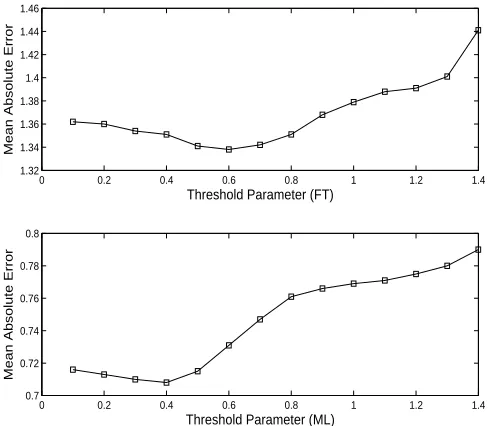
6.1.3 Optimal Value ofβ
For determining the optimal value ofβ, wee keptα= 0.25 and α= 0.1 for MovieLens and FilmTrust dataset, and varied the value ofβ from 0 to 1.4 with a difference of 0.1. The results are shown in figure 2. Figure 2 shows that
α= 0.4 andα= 0.6 gave the lowest MAE for MovieLens and FilmTrust dataset respectively.
23
0 0.2 0.4 0.6 0.8 1 1.2 1.4 1.32
1.34 1.36 1.38 1.4 1.42 1.44 1.46
Threshold Parameter (FT)
Mean Absolute Error
0 0.2 0.4 0.6 0.8 1 1.2 1.4
0.7 0.72 0.74 0.76 0.78 0.8
Threshold Parameter (ML)
Mean Absolute Error
Figure 3: Determining the optimal value ofβ.
6.2
Performance Evaluation With Other
Al-gorithms
6.2.1 Performance Evaluation in Terms of MAE, ROC-Sensitivity, and Coverage
Table 1 shows the on-line cost24
of algorithms with their respective MAE, ROC-sensitivity, and coverage. We show the best results and the results of proposed algo-rithm in bold. Here, f is the number of features/words in the dictionary (used in Naive Bayes classifier). It is worth noting that for FilmTrust dataset, ROC sensitiv-ity is lower, for all algorithms in general, as compared to the MovieLens dataset. We believe that it is due to the rating distribution. Furthermore, the coverage of the al-gorithms is much lower in the case of FilmTrust dataset, which is due to the reason that it is very sparse (99%). The table depicts that the proposed algorithm is scalable and practical as its on-line cost is less or equal to the cost of other algorithms.
Table 1 shows that the proposed algorithm outperforms other significantly in terms of MAE, ROC-sensitivity, and coverage. It is because, when Naive Bayes classifier has sufficiently large confidence in prediction, then it can cor-rectly classify an instance (a unknown rating). In our case, Naive Bayes classifier was able to accurately pre-dict about 40% and 36% ratings of the test set in the case of MovieLens and FilmTrust dataset respectively, resulting in the reduced MAE, increased ROC-sensivity and coverage.
24
[image:8.595.48.292.73.286.2]It is the cost for generating predictions forNitems. We assume we compute item similarities and train Naive Bayes classifier in off-line fashion.
Table 2: Performance evaluation in new item cold-start problem
Algo. MAE0 MAE2 MAE5
(ML) (FT) (ML) (FT) (ML) (FT)
U BCFDV – – 1.235 2.223 0.932 1.825
IBCF – – 1.209 2.172 0.873 1.764 IDemo4 – – 1.191 2.162 0.852 1.682 CB 0.831 1.481 0.821 1.456 0.811 1.448
RecN BCF 0.822 1.459 0.818 1.452 0.809 1.451
6.2.2 Performance Evaluation Under Cold-Start Scenarios
We checked the performance of the algorithm under new item cold-start problems25
. When an item is rated by only few users, then item-based and user-based CF will not give us good results. Our proposed scheme works well in new item cold-start problem scenario, as it does not solely depend on the number of users who have rated the target item for finding the similarity. For testing our algorithm in this scenario, we selected 1000 random sam-ples of user/item pairs from the test set. While making prediction for a target item, the number of users in the training set who have rated target item were kept 0, 2, and 5. The correspondingMAE; represented byMAE0, MAE2,MAE5, is shown in table 2.
Table 2 shows that CF and IDemo4 fail to make predic-tion when only the active user rated the target item, and in general they gave inaccurate predictions. It is worth noting that, in e-commerce domains (e.g. Amazon), there may be millions of items that are rated by only a few users (<5). In this scenario, CF and related approaches would results in inaccurate recommendations. The poor performance of user-based CF is due to the reason that, we have less neighbours against an active user, hence per-formance degrades. The reason in case of item-based CF is that, the similar items found after applying rating cor-relation may be not actually similar. As while finding similarity, we isolate all users who have rated both target item and the item we find similarity with. In this case, we have maximum 5 users who have rated both items, as a result, similarity found by adjusted cosine measure will be misleading. The IDemo4 produces poor results, as it operates over candidate neighbouring items found after applying the rating similarity. Both content-boosted and
RecN BCF make effective use of user’s content profile that
can be used by a classifier for making predictions.
25
6.2.3 Performance Evaluation In Terms of Cost
The cost of the proposed algorithm is given in table 1. We are using item-based CF, whose on-line cost is less than that of user-based CF used in [20]26
. Even if we consider using naive Bayes classifier to fill the user-item rating ma-trix and then use item-based CF over this filled mama-trix, then our cost will be less than that. The reason is in the filled matrix case, one has to go through all the filled rows of matrix for finding the similar items. For a large e-commerce system like Amazon, where we already have millions of neighbours against an active user/item, filling the matrix and then going through all the users/items for finding the similar users/items in not pragmatic due to limited memory and other constraint on the execution time of the recommender system.
7
Conclusion And Future Work
In this paper, we have proposed a switching hybrid rec-ommendation approach by combining item-based collab-orative filtering with a Naive Bayes classifier. We em-pirically show that our recommendation approach out-perform others in terms of accuracy, and coverage and is more scalable. As a future work, we would like to apply Support Vector Machines over features vectors for gener-ating recommendations. Furthermore, we would like to evaluate our algorithms on dataset of domains other than movies, such as BookCrossing27
dataset.
Acknowledgment
The work reported in this paper has formed part of the Instant Knowledge Research Programme of Mobile VCE, (the Virtual Centre of Excellence in Mobile & Personal Communications), www.mobilevce.com. The programme is co-funded by the UK Technology Strategy Boards Col-laborative Research and Development programme. De-tailed technical reports on this research are available to all Industrial Members of Mobile VCE. We would like to thank Juergen Ulbts (http://www.jmdb.de/) and Martin Helmhout for helping integrating datasets with IMDB.
References
[1] P. Resnick and H. R. Varian, “Recommender sys-tems,” Commun. ACM, vol. 40, no. 3, pp. 56–58, 1997.
[2] B. Mobasher, “Recommender systems,” Kunstliche Intelligenz, Special Issue on Web Mining, vol. 3, pp. 41–43, 2007.
26
It is because, we can build expensive and less volatile item similarity model in off-line fashion. Hence on-line cost becomes O(N2
) in worst case, and in practical it isO(KN), whereKis the number of topKmost similar items against a target item (K < N).
27
http://www.informatik.uni-freiburg.de/ cziegler/BX/
[3] J. Y. G Linden, B Smith, “Amazon.com recom-mendations: item-to-item collaborative filtering,” in IEEE, Internet Computing, vol. 7, 2003, pp. 76–80.
[4] D. Goldberg, D. Nichols, B. Oki, and D. Terry, “Us-ing collaborative filter“Us-ing to weave an information tapestry,” Communications of the ACM, vol. 35, no. 12, p. 70, 1992.
[5] U. Shardanand and P. Maes, “Social information fil-tering:algorithms for automating word of mouth,” in Proc. Conf. Human Factors in Computing Systems, 1995, pp. 210–217.
[6] L. Terveen, W. Hill, B. Amento, D. McDonald, and J. Creter, “Phoaks: A system for sharing recommen-dations,” inComm. ACM, vol. 40, 1997, pp. 59–62.
[7] P. Resnick, N. Iacovou, M. Suchak, P. Bergstrom, and J. Riedl, “GroupLens: An open architecture for collaborative filtering of netnews,” inProceedings of the 1994 ACM conference on Computer supported cooperative work. ACM New York, NY, USA, 1994, pp. 175–186.
[8] J. A. Konstan, B. N. Miller, D. Maltz, J. L. Her-locker, L. R. Gordon, and J. Riedl, “Grouplens: ap-plying collaborative filtering to usenet news,” Com-mun. ACM, vol. 40, no. 3, pp. 77–87, March 1997.
[9] A. T. Gediminas Adomavicius, “Toward the next generation of recommender systems: A survey of the state-of-the-art and possible extensions,” IEEE Transactions on Knowledge and Data Engineering, vol. 17, pp. 734–749, 2005.
[10] B. Sarwar, G. Karypis, J. Konstan, and J. Reidl, “Item-based collaborative filtering recommendation algorithms,” inProceedings of the 10th international conference on World Wide Web. ACM New York, NY, USA, 2001, pp. 285–295.
[11] B. Sarwar, G. Karypis, J. Konstan, and J. Riedl, “Application of dimensionality reduction in recom-mender system–a case study,” in ACM WebKDD 2000 Web Mining for E-Commerce Workshop. Cite-seer, 2000.
[12] J. S. Breese, D. Heckerman, and C. Kadie, “Empiri-cal analysis of predictive algorithms for collaborative filtering.” Morgan Kaufmann, 1998, pp. 43–52.
[13] Y. Park and A. Tuzhilin, “The long tail of recom-mender systems and how to leverage it,” in Proceed-ings of the 2008 ACM conference on Recommender systems. ACM New York, NY, USA, 2008, pp. 11– 18.
[15] K. Lang, “Newsweeder: Learning to filter netnews,” in In Proceedings of the Twelfth International Con-ference on Machine Learning, 1995.
[16] S. Alag,Collective Intelligence in Action. Manning Publications, October, 2008.
[17] S. Al Mamunur Rashid, G. Karypis, and J. Riedl, “ClustKNN: a highly scalable hybrid model-& memory-based CF algorithm,” inProc. of WebKDD 2006: KDD Workshop on Web Mining and Web Us-age Analysis, August 20-23 2006, Philadelphia, PA. Citeseer.
[18] R. Burke, “Hybrid recommender systems: Survey and experiments,”User Modeling and User-Adapted Interaction, vol. 12, no. 4, pp. 331–370, November 2002.
[19] M. J. Pazzani, “A framework for collaborative, content-based and demographic filtering,”Artificial Intelligence Review, vol. 13, no. 5 - 6, pp. 393–408, December 1999.
[20] P. Melville, R. J. Mooney, and R. Nagarajan, “Content-boosted collaborative filtering for im-proved recommendations,” inin Eighteenth National Conference on Artificial Intelligence, 2002, pp. 187– 192.
[21] R. J. Mooney and L. Roy, “Content-based book rec-ommending using learning for text categorization,” in Proceedings of DL-00, 5th ACM Conference on Digital Libraries. San Antonio, US: ACM Press, New York, US, 2000, pp. 195–204.
[22] M. Vozalis and K. Margaritis, “Collaborative filter-ing enhanced by demographic correlation,” inAIAI Symposium on Professional Practice in AI, of the 18th World Computer Congress, 2004.
[23] ——, “On the enhancement of collaborative filtering by demographic data,”Web Intelligence and Agent Systems, vol. 4, no. 2, pp. 117–138, 2006.
[24] Y. S. Marko Balabanovic, “Fab: content-based, col-laborative recommendation,” inCommunications of the ACM archive, vol. 40, Miami, Florida, USA, 1997, pp. 66–72.
[25] M. Claypool, A. Gokhale, T. Mir, P. Murnikov, D. Netes, and M. Sartin, “Combining content-based and collaborative filters in an online newspaper,” in In Proceedings of ACM SIGIR Workshop on Recom-mender Systems, 1999.
[26] H. Ma, I. King, and M. Lyu, “Effective missing data prediction for collaborative filtering,” inProceedings of the 30th annual international ACM SIGIR con-ference on Research and development in information retrieval. ACM, 2007, p. 46.
[27] U. Nahm and R. Mooney, “Text mining with infor-mation extraction,” 2002.
[28] K. Aas and L. Eikvil, “Text categorisation: A sur-vey.” 1999.
[29] I. H. W. Witten and F. Eibe, Data Mining: Prac-tical Machine Learning Tools and Techniques with Java Implementations. Morgan Kaufmann, Octo-ber 1999.
[30] K. JUNG and J. LEE, “User Preference Min-ing through Hybrid Collaborative FilterMin-ing and Content-based Filtering in Recommendation Sys-tem,”IEICE TRANSACTIONS on Information and Systems, vol. 87, no. 12, pp. 2781–2790, 2004.
[31] M. Vozalis and K. Margaritis, “Using SVD and de-mographic data for the enhancement of generalized collaborative filtering,” Information Sciences, vol. 177, no. 15, pp. 3017–3037, 2007.
[32] L. G. T. Jonathan L. Herlocker, Joseph A. Konstan and J. T. Riedl, “Evaluating collaborative filtering recommender systems,” ACM Transactions on In-formation Systems (TOIS) archive, vol. 22, pp. 734– 749, 2004.
[33] B. M. Sarwar, G. Karypis, J. Konstan, and J. Riedl, “Recommender systems for large-scale e-commerce: Scalable neighborhood formation using clustering,” 2002.
[34] B. Sarwar, G. Karypis, J. Konstan, and J. Riedl, “Analysis of recommendation algorithms for e-commerce.” ACM Press, 2000, pp. 158–167.
![Table 1: A comparison of proposed algorithm with existing in terms of cost (based on [31]), accuracy metrics, andcoverage](https://thumb-us.123doks.com/thumbv2/123dok_us/1305105.660337/7.595.50.556.106.448/table-comparison-proposed-algorithm-existing-accuracy-metrics-andcoverage.webp)