Fast Mapping in Word Learning: What Probabilities Tell Us
Afra Alishahi and Afsaneh Fazly and Suzanne Stevenson Department of Computer Science
University of Toronto
{afra,afsaneh,suzanne}@cs.toronto.edu
Abstract
Children can determine the meaning of a new word from hearing it used in a familiar context—an ability often referred to as fast
mapping. In this paper, we study fast
map-ping in the context of a general probabilistic model of word learning. We use our model to simulate fast mapping experiments on chil-dren, such as referent selection and retention. The word learning model can perform these tasks through an inductive interpretation of the acquired probabilities. Our results suggest that fast mapping occurs as a natural conse-quence of learning more words, and provides explanations for the (occasionally contradic-tory) child experimental data.
1 Fast Mapping
An average six-year-old child knows over 14,000 words, most of which s/he has learned from hearing other people use them in ambiguous contexts (Carey, 1978). Children are thus assumed to be equipped with powerful mechanisms for performing such a complex task so efficiently. One interesting ability children as young as two years of age show is that of correctly and immediately mapping a novel word to a novel object in the presence of other familiar objects. The term “fast mapping” was first used by Carey and Bartlett (1978) to refer to this phenomenon.
Carey and Bartlett’s goal was to examine how much children learn about a word when presented in an am-biguous context, as opposed to concentrated teaching. They used an unfamiliar name (chromium) to refer to an unfamiliar color (olive green), and then asked a group of four-year-old children to select an object from among a set, upon hearing a sentence explicitly
c
2008. Licensed under the Creative Commons Attribution-Noncommercial-Share Alike 3.0 Unported li-cense (http://creativecommons.org/lili-censes/by-nc-sa/3.0/). Some rights reserved.
asking for the object of the new color, as in: bring
the chromium tray, not the blue one. Children were
generally good at performing this “referent selection” task. In a production task performed six weeks later, when children had to use the name of the new color, they showed signs of having learned something about the new color name, but were not successful at pro-ducing it. On the basis of these findings, Carey and Bartlett suggest that fast mapping and word learning are two distinct, yet related, processes.
Extending Carey and Bartlett’s work, much re-search has concentrated on providing an explanation for fast mapping, and on examining its role in word learning. These studies also show that children are generally good at referent selection, given a novel tar-get. However, there is not consistent evidence regard-ing whether children actually learn the novel word from one or a few such exposures (retention). For example, whereas the children in the experiments of Golinkoff et al. (1992) and Halberda (2006) showed signs of nearly-perfect retention of the fast-mapped words, those in the studies reported by Horst and Samuelson (2008) did not (all participating children were close in age range).
There are also many speculations about the possible causes of fast mapping. Some researchers consider it as a sign of a specialized (innate) mechanism for word learning. Markman and Wachtel (1988), for ample, argue that children fast map because they ex-pect each object to have only one name (mutual exclu-sivity). Golinkoff et al. (1992) attribute fast mapping to a (hard-coded) bias towards mapping novel names to nameless object categories. Some even suggest a change in children’s learning mechanisms, at around the time they start to show evidence of fast mapping (which coincides with a sudden burst in their vocab-ulary), e.g., from associative to referential (Gopnik and Meltzoff, 1987; Reznick and Goldfield, 1992). In contrast, others see fast mapping as a phenomenon that arises from more general processes of learning
and/or communication, which also underlie the im-pressive rate of lexical acquisition in children (e.g., Clark, 1990; Diesendruck and Markson, 2001; Regier, 2005; Horst et al., 2006; Halberda, 2006).
In our previous work (Fazly et al., 2008), we pre-sented a word learning model which proposes a prob-abilistic interpretation of cross-situational learning, and bootstraps its own partially-learned knowledge of the word meanings to accelerate word learning over time. We have shown that the model can learn reason-able word–meaning associations from child-directed data, and that it accounts for observed learning pat-terns in children, such as vocabulary spurt, without requiring a developmental change in the underlying learning mechanism. Here, we use this computational model to investigate fast mapping and its relation to word learning. Specifically, we take a close look at the onset of fast mapping in our model by simulat-ing some of the psychological experiments mentioned above. We examine the behaviour of the model in var-ious referent selection and retention tasks, and pro-vide explanations for the (occasionally contradictory) experimental results reported in the literature. We also study the effect of exposure to more input on the per-formance of the model in fast mapping.
Our results suggest that fast mapping can be ex-plained as an induction process over the acquired as-sociations between words and meanings. Our model learns these associations in the form of probabilities within a unified framework; however, we argue that different interpretations of such probabilities may be involved in choosing the referent of a familiar as op-posed to a novel target word (as noted by Halberda, 2006). Moreover, the overall behaviour of our model confirms that the probabilistic bootstrapping approach to word learning naturally leads to the onset of fast mapping in the course of lexical development, with-out hard-coding any specialized learning mechanism into the model to account for this phenomenon.
2 Overview of the Computational Model
This section summarizes the model presented in Fa-zly et al. (2008). Our word learning algorithm is an adaptation of the IBM translation model proposed by Brown et al. (1993). However, our model is incre-mental, and does not require a batch process over the entire data.
2.1 Utterance and Meaning Representations
The input to our word learning model consists of a set of utterance–scene pairs that link an observed scene (what the child perceives) to the utterance that de-scribes it (what the child hears). We represent each utterance as a sequence of words, and the
correspond-ing scene as a set of meancorrespond-ing symbols. To simulate
referential uncertainty (i.e., the case where the child
perceives aspects of the scene that are unrelated to the perceived utterance), we include additional symbols in the representation of the scene, e.g.:
Utterance: Joe rolled the ball
Scene:{joe,roll,the,ball,mommy,hand,talk}
In Section 3.1, we explain how the utterances and the corresponding semantic symbols are selected, and how we add referential uncertainty.
Given a corpus of such utterance–scene pairs, our model learns the meaning of each wordwas a prob-ability distribution, p(.|w), over the semantic sym-bols appearing in the corpus. In this representation, p(m|w) is the probability of a symbol m being the meaning of a wordw. In the absence of any prior knowledge, all symbols are equally likely to be the meaning of a word. Hence, prior to receiving any us-ages of a given word, the model assumes a uniform distribution over semantic symbols as its meaning.
2.2 Meaning Probabilities
Our model combines probabilistic interpretations of cross-situational learning (Quine, 1960) and of a variation of the principle of contrast (Clark, 1990), through an interaction between two types of prob-abilistic knowledge acquired and refined over time. Given an utterance–scene pair received at timet, i.e., (U(t),S(t)), the model first calculates an alignment
probability a for each w∈U(t) and each m∈S(t), using the meaning probabilities p(.|w) of all the words in the utterance prior to this time. The model then revises the meaning of the words inU(t)by in-corporating the alignment probabilities for the current input pair. This process is repeated for all the input pairs, one at a time.
Step 1: Calculating the alignment probabilities. We estimate the alignment probabilities of words and meaning symbols based on a localized version of the principle of contrast: that a meaning sym-bol in a scene is likely to be highly associated with only one of the words in the corresponding
utter-ance.1 For a symbolm∈S(t) and a wordw∈U(t), the higher the probability of m being the meaning of w (according to p(m|w)), the more likely it is that m is aligned with w in the current input. In other words, a(w|m, U(t),S(t)) is proportional to
p(t−1)(m|w). In addition, if there is strong evidence
that m is the meaning of another word in U(t)— i.e., ifp(t−1)(m|w′)is high for somew′∈U(t)other
1Note that this differs from what is widely known as the
thanw—the likelihood of aligningmtowshould de-crease. Combining these two requirements:
a(w|m,U(t),S(t)) = Xp(t−1)(m|w)
w′∈U(t)
p(t−1)(m|w′) (1)
Due to referential uncertainty, some of the meaning symbols in the scene might not have a counterpart in the utterance. To accommodate for such cases, a dummy word is added to each utterance before the alignment probabilities are calculated, in order to let a meaning symbol not be (strongly) aligned with any of the words in the current utterance.
Step 2: Updating the word meanings. We need to update the probabilitiesp(.|w)for all wordsw∈U(t), based on the evidence from the current input pair re-flected in the alignment probabilities. We thus add the current alignment probabilities forwand the sym-bolsm∈S(t)to the accumulated evidence from prior co-occurrences of w and m. We summarize this cross-situational evidence in the form of an associa-tion score, which is updated incrementally:
assoc(t)(w, m) = assoc(t−1)(w, m) +
a(w|m,U(t), S(t)) (2)
whereassoc(t−1)(w, m)is zero ifwandmhave not co-occurred before. The association score of a word and a symbol is basically a weighted sum of their co-occurrence counts.
The model then uses these association scores to up-date the meaning of the words in the current input:
p(t)(m|w) = X assoc(t)(m, w) +λ
mj∈M
assoc(t)(m
j,w) + β×λ
(3)
whereMis the set of all symbols encountered prior to or at timet,βis the expected number of symbol types, andλis a small smoothing factor. The denominator is a normalization factor to get valid probabilities. This formulation results in a uniform probability of 1/β over allm∈ Mfor a novel wordw, and a probability smaller thanλfor a meaning symbolmthat has not been previously seen with a familiar wordw.
Our model updates the meaning of a word ev-ery time it is heard in an utterance. The strength of learning of a word at time t is reflected in p(t)(m=mw|w), where mw is the “correct”
mean-ing ofw: for a learned word w, the probability dis-tributionp(.|w)is highly skewed towards the correct meaningmw, and therefore hearingwwill trigger the retrieval of the meaningmw.2
2An input-generation lexicon contains the correct meaning for
each word, as described in Section 3.1. Note that the model does not have access to this lexicon for learning; it is used only for input generation and evaluation.
From this point on, we simply usep(m|w) (omit-ting the superscript(t)) to refer to the meaning prob-ability ofmforwat the present time of learning.
2.3 Referent Probabilities
The meaning probability p(m|w) is used to retrieve the most probable meaning forwamong all the possi-ble meaning symbolsm. However, in the referent se-lection tasks performed by children, the subject is of-ten forced to select the referent of a target word from among a limited set of objects, even when the mean-ing of the target word has not been accurately learned yet. For our model to perform such tasks, it has to de-cide how likely it is for a target wordwto refer to a particular objectm, based on its previous knowledge about the mapping betweenmandw(i.e., p(m|w)), as well as the mapping betweenmand other words in the lexicon.3
The likelihood of using a particular namewto refer to a given objectmis calculated as:
rf(w|m) = p(w|m) = p(m|p(m)w)·p(w)
= P p(m|w)·p(w)
w′∈Vp(m|w′)·p(w′) (4)
whereVis the set of all words that the model has seen so far, andp(w)is the relative frequency ofw:
p(w) = P freq(w) w′∈Vfreq(w′)
(5)
The referent of a target wordwamong the present ob-jects, therefore, will be the objectmwith the highest referent probabilityrf(w|m).
3 Experimental Setup
3.1 The Input Corpora
We extract utterances from the Manchester corpus (Theakston et al., 2001) in the CHILDES database (MacWhinney, 2000). This corpus contains tran-scripts of conversations with children between the ages of 1; 8 and 3; 0 (years;months). We use the mother’s speech from transcripts of 6 children, re-move punctuation and lemmatize the words, and con-catenate the corresponding sessions as input data.
There is no semantic representation of the corre-sponding scenes available from CHILDES. There-fore, we automatically construct a scene representa-tion for each utterance, as a set containing the seman-tic referents of the words in that utterance. We get these from an input-generation lexicon that contains a symbol associated with each word as its semantic
3All through the paper, we usemas both the meaning and the
referent. We use every other sentence from the orig-inal corpus, preserving their chronological order. To simulate referential uncertainty in the input, we then pair each sentence with its own scene representation as well as that of the following sentence in the origi-nal corpus. (Note that the latter sentence is not used as an utterance in our input.) The extra semantic sym-bols that are added to each utterance thus correspond to meaningful semantic representations, as opposed to randomly selected symbols. In the resulting corpus of92,239input pairs, each utterance is, on average, paired with78%extra meaning symbols, reflecting a high degree of referential uncertianty.
3.2 The Model Parameters
We set the parameters of our learning algorithm using a development data set which is similar to our training and test data, but is selected from a non-overlapping portion of the Manchester corpus. The expected num-ber of symbols,βin Eq. (3), is set to8500based on the total number of distinct symbols extracted for the development data. Therefore, the default probability of a symbol for a novel word will be1/8500. A famil-iar word, on the other hand, has been seen with some symbols before. Therefore, the probability of a previ-ously unseen symbol for it (which, based on Eq. (3), has an upper bound ofλ) must be less than the default probability mentioned above. Accordingly, we setλ to10−5.
3.3 The Training Procedure
In the next section, we report results from the com-putational simulation of our model for a number of experiments. All of the simulations use the same pa-rameter settings (as described in the previous section), but different input: in each simulation, a random por-tion of 1000 utterance–scene pairs is selected from the input corpus, and incrementally processed by the model. The size of the training corpus is chosen arbi-trarily to reflect a sample point in learning, and further experiments have shown that increasing this number does not change the pattern observed in the results. In order to avoid behaviour that is specific to a particu-lar sequence of input items, the reported results in the next section are averaged over10simulations.
4 Experimental Results and Analysis
4.1 Referent Selection
In a typical word learning scenario, the child faces a scene where a number of familiar and unfamiliar objects are present. The child then hears a sentence, which describes (some part of) the scene, and is com-posed of familiar and novel words (e.g., hearing Joe is
eating a cheem, where cheem is a previously unseen
fruit). In such a setting, our model aligns the objects in the scene with the words in the utterance based on its acquired knowledge of word meanings, and then updates the meanings of the words accordingly. The model can align a familiar word with its referent with high confidence, since the previously learned mean-ing probability of the familiar object given the famil-iar word, orp(m|w), is much higher than the meaning probability of the same object given any other word in the sentence. In a similar fashion, the model can eas-ily align a novel word in the sentence with a novel object in the scene, because the meaning probability of the novel object given the novel word (1/β, ac-cording to Eq. (3)) is higher than the meaning proba-bility of that object for any previously heard word in the sentence (the latter probability is smaller thanλin Eq. (3), as explained in Section 3.2).
Earlier fast mapping experiments on children as-sumed that it is such a contrast between the familiar and novel words in the same sentence that helps chil-dren select the correct target object in a referent selec-tion task. For example, in Carey and Bartlett’s (1978) experiment, to introduce a novel word–meaning as-sociation (e.g., chromium–olive), the authors use both the familiar and the novel words in one sentence (bring me the chromium tray, not the blue one.). How-ever, further experiments show that children can suc-cessfully select the correct referent even if such a con-trast is not present in the sentence. Many researchers have performed experiments where young subjects are forced to choose between a novel and a familiar object upon hearing a request, such as give me the
ball (familiar target), or give me the dax (novel
tar-get). In all of the reported experimental results, chil-dren can readily pick the correct referent for a famil-iar or a novel target word in such a setting (Golinkoff et al., 1992; Halberda and Goldman, 2008; Halberda, 2006; Horst and Samuelson, 2008).
However, Halberda’s eye-tracking experiments on both adults and pre-schoolers suggest that the pro-cesses involved for referent selection in the familiar target situation may be different from those in the novel target situation. In the latter situation, subjects appear to systematically reject the familiar object as the referent of the novel name before mapping the novel object to the novel name. In the familiar target situation, however, there is no need to reject the novel distractor object, because the subject already knows the referent of the target.
“get the ball” while facing aballand a novel object (dax). We assume that the child knows the meaning of verbs and determiners such as get and the, therefore we simplify the familiar target condition in the form of the following input item:
ball (FAMILIARTARGET) {ball,dax}
A familiar word such as ball has a meaning prob-ability highly skewed towards its correct meaning. That is, upon hearing ball, the model can confidently retrieve its meaning ball, which is the one with the highest probabilityp(m|ball)among all possible meaningsm. In such a case, ifballis present in the scene, the model can easily pick it as the referent of the familiar target name, without processing the other objects in the scene.
Now consider the condition where a novel target name is used in the presence of a familiar and a pre-viously unseen object:
dax (NOVELTARGET)
{ball,dax}
Since this is the first time the model has heard the word dax, both meaningsballanddaxare equally likely because p(.|dax)is uniform. Thus the mean-ing probabilities cannot be solely used for selectmean-ing the referent of dax, and the model has to perform some kind of induction on the potential referents in the scene based on what it has learned about each of them. The model can infer the referent of dax by comparing the referent probabilitiesrf(dax|ball) andrf(dax|dax)from Eq. (4) after processing the in-put item. Sinceballhas strong associations with an-other word ball, its referent probability for the novel name dax is much lower than the referent probability ofdax, which does not have strong associations with any of the words in the learned lexicon.
We simulate the process of referent selection in our model as follows. We train the model as described in Section 3.3. We then present the model with one more input item, which represents either the FAMIL
-IAR TARGETor the NOVEL TARGET condition. For each condition, we compare the meaning probability p(object|target)for both familiar and novel objects in the scene (see Table 1, top panel). In the FA
-MILIAR TARGET condition, the model demonstrates a strong preference towards choosing the familiar ob-ject as the referent, whereas in the NOVEL TARGET
condition, the model shows no preference towards any of the objects based on the meaning probabilities of the target word. Therefore, for the NOVEL TARGET
condition, we also compare the referent probabilities
rf(target|object)for both objects after processing
Table 1: Referent selection in FAMILIARand NOVEL
TARGETconditions.
UPON HEARING THE TARGET WORD
Condition p(ball|target) p(dax|target) FAMILIARTARGET 0.843±0.056 ≪0.0001
NOVELTARGET 0.0001±0.00 0.0001±0.00
AFTER PERFORMING INDUCTION
Condition rf(target|ball) rf(target|dax) NOVELTARGET 0.127±0.127 0.993±0.002
the input item as a training pair, simulating the in-duction process that humans go through to select the referent in such cases. This time, the model shows a strong preference towards the novel object as the ref-erent of the target word (see Table 1, bottom panel). Our results confirm that in both conditions, the model consistently selects the correct referent for the target word across all the simulations.
4.2 Retention
As discussed in the previous section, results from the human experiments as well as our computational simulations show that the referent of a novel target word can be selected based on the previous knowl-edge about the present objects and their names. How-ever, the success of a subject in a referent selection task does not necessarily mean that the child/model has learned the meaning of the novel word based on that one trial. In order to better understand what and how much children learn about a novel word from a single ambiguous exposure, some studies have per-formed retention trials after the referent selection ex-periments. Often, various referent selection trials are performed in one session, where in each trial a novel object–name pair is introduced among familiar ob-jects. Some of the recently introduced objects are then put together in one last trial, and the subjects are asked to choose the correct referent for one of the (recently heard) novel target words. The majority of the reported experiments show that children can suc-cessfully perform the retention task (Golinkoff et al., 1992; Halberda and Goldman, 2008; Halberda, 2006). We simulate a similar retention experiment by training the model as usual. We further present the model with two experimental training items similar to the one used in the NOVELTARGETcondition in the previous section, with different familiar and novel ob-jects and words in each input:
dax (REFERENTSELECTIONTRIAL1) {ball,dax}
Table 2: Retention of a novel target word from a set of novel objects.
2-OBJECTRETENTIONTRIAL rf(dax|dax) rf(dax|cheem)
0.996±0.001 0.501±0.068
3-OBJECTRETENTIONTRIAL rf(dax|dax) rf(dax|cheem) rf(dax|lukk)
0.995±0.001 0.407±0.062 0.990±0.001
The training session is followed by a retention trial, where the two novel objects used in the previous ex-perimental inputs are paired with one of the novel tar-get words:
dax (2-OBJECTRETENTIONTRIAL) {cheem,dax}
After processing the retention input, we com-pare the referent probabilities rf(dax|cheem) and
rf(dax|dax)to see if the model can choose the cor-rect novel object in response to the target word dax. The top panel in Table 2 summarizes the results of this experiment. The model consistently shows a strong preference towards the correct novel object as the ref-erent of the novel target word across all simulations.
Unlike studies on referent selection, experimental results for retention have not been consistent across various studies. Horst and Samuelson (2008) per-form experiments with two-year-old children involv-ing both referent selection and retention, and report that their subjects perform very poorly at the retention task. One factor that discriminates the experimental setup of Horst and Samuelson from others (e.g., Hal-berda, 2006) is that, in their retention trials, they put together two recently observed novel objects with a third novel object that has not been seen in any of the experimental sessions before. The authors do not at-tribute their contradictory results to the presence of this third object, but this factor can in fact affect the performance considerably. We simulate this condition by using the same input items for referent selection trials as in the previous simulation, but we replace the retention trial with the following:
dax (3-OBJECTRETENTIONTRIAL) {cheem,dax,lukk}
The third object, lukk, has not been seen by the model before. Results under the new condition are re-ported in the bottom panel of Table 2. As can be seen, the model shows a strong tendency towards the cor-rect novel referentdaxfor the novel target dax, com-pared to the other recently seen novel objectcheem. However, the probability of the unseen object lukk is also very high for the target word dax. That is be-cause the model cannot use any previously acquired
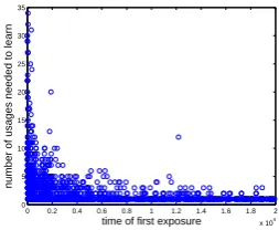
0 0.2 0.4 0.6 0.8 1 1.2 1.4 1.6 1.8 2 x 10⁴
0 5 10 15 20 25 30 35
time of first exposure
[image:6.595.92.279.121.191.2]number of usages needed to learn
Figure 1: Number of usages needed to learn a word, as a function of the word’s age of exposure.
knowledge about lukk (i.e., associating it with an-other word) to rule it out as a referent for dax. These results show that introducing a new object for the first time in a retention trial considerably increases the dif-ficulty of the task. This can explain the contradictory results reported in the literature: when the referent probabilities are not informative, other factors may influence the outcome of the experiment, such as the amount of training received for a novel word–object, or a possible delay between training and test sessions.
4.3 The Effect of Exposure to More Input
The fast mapping ability observed in children implies that once children have learned a repository of words, they can easily link novel words to novel objects in a familiar context based only on a few exposures. We examine this effect in our model: we train the model on20,000input pairs, looking at the relation between the time of first exposure to a word, and the number of usages that the model needs for learning that word. Figure 1 plots this for words that have been learned at some point during the training.4 We can see that the model shows clear fast mapping behaviour—that is, words received later in time, on average, require fewer usages to be learned. These results show that our model exhibits fast mapping patterns once it has been exposed to enough word usages, and that no change in the underlying learning mechanism is needed.5
The effect of exposure to more input on fast map-ping can be described in terms of context familiarity: the more input the model has processed so far, the more likely it is that the context of the usage of a novel word (the other words in the sentence and the objects in the scene) is familiar to the model. This pattern has been studied through a number of experiments on
4We consider a wordwas learned if the meaning probability p(mw|w)is higher than a certain thresholdθ. For this experi-ment, we setθ= 0.70.
5In Fazly et al. (2008), we reported a variation of this
children. For example, Gershkoff-Stowe and Hahn (2007) taught16- to18-month-olds the names of24 unfamiliar objects over 12 training sessions, where unfamiliar objects were presented with varying fre-quency. Data were compared to a control group of children who were exposed to the same experimen-tal words at the first and last sessions only. Their re-sults show that for children in the experimental group, extended practice with a novel set of words led to the rapid acquisition of a second set of low-practice words. Children in the control group did not show the same lexical advantage.
Inspired by Gershkoff-Stowe and Hahn (2007), we perform an experiment to study the effect of con-text familiarity on fast mapping in our model. We choose two sets of words, CONTEXT (containing 20 words) and TARGET (containing 10 words), to con-duct a referent selection task as follows. First, we train our model on a sequence of utterance–scene pairs constructed from the set CONTEXT∪TARGET, as follows: the unified set is randomly shuffled and divided into two subsets, words in each subset are put together to form an utterance, and the meanings of the words in that utterance are put together to form the corresponding scene. We repeat this process twice, so that each word appears in exactly two input pairs. We train our model on the constructed pairs.6 Next, we perform a referent selection task on each word in the TARGET set: we pair each target word wwith the meaning of 10randomly selected words from CONTEXT∪TARGET, including the meaning of
the target word itself (mw), and have the model pro-cess this test pair. We compare the referent probabil-ity ofw and eachm∈CONTEXT∪TARGET to see whether the model can correctly map the target word to its referent. We call this setting the LOWTRAIN
-INGcondition.
In the above setting, the context words in the ref-erent selection trials are as new to the model as the target words. We thus repeat this experiment with a familiar context: we first train the model over in-put pairs that are randomly constructed from words in CONTEXT only, using the same training
proce-dure as described above. This context-familiarization process is followed by a similar training session on CONTEXT∪TARGET, and a test session on target words, similar to the previous condition. Again, we count the number of correct mappings between a tar-get word and its referent based on the referent proba-bilities. We call this setting the HIGHTRAINING con-dition. Table 3 shows the results for both conditions. It can be seen that the accuracy of finding the referent
6Unlike in previous experiments, here we do not use
child-directed data as we want to control the familiarity of the context.
Table 3: Average number of correct mappings and the referent probabilities of target words for two condi-tions, LOWand HIGHTRAINING.
Condition Correct mappings P(target|mtarget) LOWTRAINING %54 0.216±0.04 HIGHTRAINING %90 0.494±0.79
for a target word, as well as the referent probability of a target word for its correct meaning, increase as a re-sult of more training on the context. In other words, a more familiar context helps the model perform better in a fast mapping task.
5 Related Computational Models
The rule-based model of Siskind (1996), and the con-nectionist model proposed by Regier (2005), both show that learning gets easier as the model is exposed to more input—that is, words heard later are learned faster. These findings confirm that fast mapping may simply be a result of learning more words, and that no explicit change in the underlying learning mech-anism is needed. However, these studies do not ex-amine various aspects of fast mapping, such as ref-erent selection and retention. Horst et al. (2006) ex-plicitly test fast mapping in their connectionist model of word learning by performing referent selection and retention tasks. The behaviour of their model matches the child experimental data reported in a study by the same authors (Horst and Samuelson, 2008), but not that of the contradictory findings of other similar ex-periments. Moreover, the model’s learning capacity is limited, and the fast mapping experiments are per-formed on a very small vocabulary. Frank et al. (2007) examine fast mapping in their Bayesian model by test-ing its performance in a novel target referent selection task. However, the experiment is performed on an ar-tifical corpus. Moreover, since the learning algorithm is non-incremental, the success of the model in refer-ent selection is determined implicitly: each possible word–meaning mapping from the test input is added to the current lexicon, and the consistency of the new lexicon is checked against the training corpus.
6 Discussion and Concluding Remarks
experimental results suggest that fast mapping can be explained as an induction process over the acquired associations between words and objects. In that sense, fast mapping is a general cognitive ability, and not a hard-coded, specialized mechanism of word learn-ing.7 In addition, our results confirm that the onset of fast mapping is a natural consequence of learning more words, which in turn accelerates the learning of new words. This bootstrapping approach results in a rapid pace of vocabulary acquisition in children, with-out requiring a developmental change in the underly-ing learnunderly-ing mechanism.
Results of the referent selection experiments show that our model can successfully find the referent of a novel target word in a familiar context. Moreover, our retention experiments show that the model can map a recently heard novel word to its recently seen novel referent (among other novel objects) after only one exposure. However, the strength of the associa-tion of a novel pair after one exposure shows a no-table difference compared to the association between a “typical” familiar word and its meaning.8 This is consistent with what is commonly assumed in the lit-erature: even though children learn something about a word from only one exposure, they often need more exposure to reliably learn its meaning (Carey, 1978). Various kinds of experiments have been performed to examine how strongly children learn novel words in-troduced to them in experimental settings. For exam-ple, children are persuaded to produce a fast-mapped word, or to use the novel word to refer to objects that are from the same category as its original refer-ent (e.g., Golinkoff et al., 1992; Horst and Samuelson, 2008). We intend to look at these new tasks in our fu-ture research.
References
Behrend, Douglas A., Jason Scofield, and Erica E. Kleinknecht 2001. Beyond fast mapping: Young chil-dren’s extensions of novel words and novel facts.
De-velopmental Psychology, 37(5):698–705.
Brown, Peter F., Stephen A. Della Pietra, Vincent J. Della Pietra, and Robert L. Mercer 1993. The mathematics of statistical machine translation: Parameter estimation.
Computational Linguistics, 19(2):263–311.
Carey, Susan 1978. The child as word learner. In Halle, M., J. Bresnan, and G. A. Miller, editors, Linguistic Theory
and Psychological Reality. The MIT Press.
Carey, Susan and Elsa Bartlett 1978. Acquiring a single new word. Papers and reports on Child Language
De-velopment, 15:17–29.
7In fact, similar fast mapping effects have been studied in
con-texts other than language. For example, Behrend et al. (2001) re-port on children’s fast mapping of novel facts about novel objects.
8After processing1000input pairs, the average meaning
prob-ability of familiar words (those with frequency higher than 10) is 0.77, whereas that of the novel word after one exposure is 0.64.
Clark, Eve 1990. On the pragmatics of contrast. Journal
of Child Language, 17:417–431.
Diesendruck, Gil and Lori Markson 2001. Children’s
avoidance of lexical overlap: A pragmatic account.
De-velopmental Psychology, 37(5):630–641.
Fazly, Afsaneh, Afra Alishahi, and Suzanne Steven-son 2008. A probabilistic incremental model of word learning in the presence of referential uncertainty. In
Proceedings of the 30th Annual Conference of the Cog-nitive Science Society.
Frank, Michael C., Noah D. Goodman, and Joshua B.
Tenenbaum 2007. A bayesian framework for
cross-situational word-learning. In Advances in Neural
Infor-mation Processing Systems, volume 20.
Gershkoff-Stowe, Lisa and Erin R. Hahn 2007. Fast map-ping skills in the develomap-ping lexicon. Journal of Speech,
Language, and Hearing Research, 50:682–697.
Golinkoff, Roberta Michnick, Kathy Hirsh-Pasek,
Leslie M. Bailey, and Neil R. Wegner 1992. Young
children and adults use lexical principles to learn new nouns. Developmental Psychology, 28(1):99–108. Gopnik, Alison and Andrew Meltzoff 1987. The
develop-ment of categorization in the second year and its relation to other cognitive and linguistic developments. Child
Development, 58(6):1523–1531.
Halberda, Justin 2006. Is this a dax which I see before me? use of the logical argument disjunctive syllogism supports word-learning in children and adults. Cognitive
Psychology, 53:310–344.
Halberda, Justin and Julie Goldman 2008. One-trial learn-ing in 2-year-olds: Children learn new nouns in 3 sec-onds flat. (in submission).
Horst, Jessica S., Bob McMurray, and Larissa K. Samuel-son 2006. Online processing is essential for learning: Understanding fast mapping and word learning in a dy-namic connectionist architecture. In Proc. of CogSci’06. Horst, Jessica S. and Larissa K. Samuelson 2008. Fast mapping but poor retention by 24-month-old infants.
In-fancy, 13(2):128–157.
MacWhinney, B. 2000. The CHILDES Project: Tools for
Analyzing Talk, volume 2: The Database. MahWah, NJ:
Lawrence Erlbaum Associates, third edition.
Markman, Ellen M. and Gwyn F. Wachtel 1988. Children’s use of mutual exclusivity to constrain the meanings of words. Cognitive Psychology, 20:121–157.
Quine, W.V.O. 1960. Word and Object. Cambridge, MA: MIT Press.
Regier, Terry 2005. The emergence of words:
Atten-tional learning in form and meaning. Cognitive Science, 29:819–865.
Reznick, J. Steven and Beverly A. Goldfield 1992. Rapid change in lexical development in comprehension and production. Developmental Psychology, 28(3):406–413.
Siskind, Jeffery Mark 1996. A computational study
of cross-situational techniques for learning word-to-meaning mappings. Cognition, 61:39–91.