Computational Solution for Rendezvous on a Line
of Four or Five Points
William H. Ruckle
∗Abstract−In a rendezvous problem on a discrete line two players are placed at points on the line. At each moment of time each player can move to an adjacent point or remain at the point at which it stands. The goal is for both players to reach the same point in the least time. There are optimal strategy pairs for which both players tend toward the center. Using this result and a matrix representation for the situation we employ a symbolic program (Maxima) to determine all possible solutions to searches on lines having four or five points, the cases of 1, 2, or 3 points being trivial.
Keywords: rendezvous, search
Introduction
We consider the problem in which two teams called Player I and Player II are placed at locations iandj respectively with probability pi,j on a discrete line. Thereafter the two players
move to adjacent locations until they finally meet by arriving at the same location. The goal is for the players to meet in the shortest time. Thus if Player I starting atichooses a path
fi and Player II starting at j chooses a path gj the goal is to
minimize the quantity
E({fi},{gj}) =
X
i,j
pi,j[fi, gj]
where [fi, gj] denotes the time before the two paths are at the
same location.
The problem described above is known as the rendezvous prob-lem on the discrete line. A description of results for this probprob-lem on the line and other lattices is described in [1], and some results for lines of arbitrary length appear in [2] and [3]. In this paper we first show that there is always an optimal pair of paths that tend toward the center. Next we show how to represent a pair of paths and its result using matrix calculations. Finally we apply the calculation to the cases of a four and five point line.
The Restriction Theorem
The main result in this section is that in every rendezvous game on the line there is always a pair of optimal strategies that are
∗Professor Emeritus, Clemson University 106 Whippoorwill Drive, Seneca,SC 29672, USA [email protected]
within increasingly shorter lines as the search proceeds. A more general theorem of this type is found in [4], but the present result is not a special case since there we defined a meeting to be in the same oradjacentlocations at the same time. It is convenient to represent the setLof locations on a line by
L={−n,−(n−1), ...,−1,0,1, ..., n}
if the line has an odd number (2n+ 1) of locations and by
L={−n,−(n−1), ...,−1,1, ..., n},
omitting 0, if the line has an even number (2n) of locations.
A path fi beginning at location i is a function from the set
of positive integers into L such that (1) fi(1) = i and (2)
fi(t+ 1)∈ {fi(t)−1, fi(t), fi(t) + 1}for each positive integer
k. We express this briefly by saying thatfi(t+ 1) isadjacent
tofi(t). Iffi andgj are two paths then [fi, gj] is the smallest
integerkfor whichfi(k) =gj(k) or∞if the paths never meet.
A pathfiis said to bekrestrictedwhere 0≤k≤nafter time
T if−k≤fi(t)≤k fort > T. Iffi is akrestricted path after
timeT we definePk−1(fi) to be the functiongfrom the positive
integers intoLdefined by
g(k) =
fi(t) ift≤T+ 1
fi(t) ift > T+ 1 and −(k−1)≤fi(t)≤k−1
k−1 ift > T + 1 andfi(t) =k
−(k−1) ift > T + 1 andfi(t) =−k
Thusgcoincides withfiuntil timeT+1 coincides withfiexcept
it stays at−(k−1) whenfigoes to −k or at (k−1) whenfi
goes tok.
Proposition 1 If fi is a k restricted path after time T then
g=Pk−1(fi)is a path that begins atiand is(k−1)restricted
after timeT+ 1as well ask restricted after timeT.
Proof. Since 1 ≤ T+ 1 it follows that g(1) =fi(1) = i. If
t≤T+ 1 or−(k−1)< fi(t)< k−1 theng(t+ 1) is adjacent
tog(t) because it coincides withfi. Ift > T+ 1 andfi(t) =k
theng(t) can be k (if t = T+ 1) or k−1 and fi(t+ 1) can
bek or k−1 sog(t+ 1) has to bek−1 which is adjacent to
g(t). If t > T+ 1 and fi(t) = k−1 then g(t) isk−1 and
fi(t+ 1) can bekork−1 sog(t+ 1) has to bek−1 which is
adjacent tog(t). We omit the similar argument forfi(t) equal
−kor−(k−1). Thatgiskrestricted after timeT follows since
Proposition 2 If fi and gj are both k restricted paths after
timeT then
[Pk−1fi, Pk−1gj]≤[fi, gj].
Proof. DenotePk−1fibyfi∗andPk−1gjbyg∗j, and let [fi, gj] =
t0. If t0 ≤T + 1 or fi(t0) ∈ {/ k,−k} thenfi∗(t0) =fi(t0) =
gj(t0) =g∗j(t0). If t0> T + 1 andfi(t0) =k thenfi∗(t0) and
g∗
i(t0) are bothk−1. Ift0> T+ 1 andfi(t0) =−kthenfi∗(t0)
and g∗
i(t0) are both−(k−1). Thusfi∗ andg
∗
i both meet at
timet0and possibly before. 2
Definition 3 A pathfi onLis calledrestricted if it isn−T
restricted after time T for T = 0,1,2, .., n−1 and fi(n) = 0
whenLhas an odd number (2n+ 1) locations orfi(n) = 1when
L has an even number (2n) locations.
Proposition 4 Iffiandgjis any pair of paths onL, there are
restricted pathsf∗
i andg
∗
j such that
f∗
i, g
∗
j
≤[fi, gj].
Proof. Sincefiandgiare paths onL, they arenrestricted so
by Proposition Pn−1fiandPn−1gjarenrestricted after time 0
andn−1 restricted after time 1 with [Pn−1fi, Pn−1gj]≤[fi, gj].
We can iterate this processn−1 times to obtain the desiredf∗
i
andg∗
i. 2
Proposition 5 Suppose PlayersI and II begin at locationsi andjrespectively with probabilitypi,j. If{fi:i∈L}is any set
of paths for Player I and {gj:j∈L} is any set of paths for
Player II then there are sets of restricted paths If {f∗
i :i∈L}
and
g∗
j :j∈L such that
X
i,j
pi,j
f∗
i, g
∗
j
≤X
i,j
pi,j[fi, gj].
Proof. For eachi, j let f∗
i, g
∗
j satisfy the conclusion of
Propo-sition 4. 2
Theorem 6 Suppose PlayersI andII begin at locationsiand j respectively with probability pi,j. There are restricted paths
{f∗
i :i∈L}and
g∗
j :j∈L such that
X
i,j
pi,jfi∗, g
∗
j
≤X
i,j
pi,j[fi, gj]
for any pair of sets of paths{fi:i∈L}and{gj:j∈L}.
Proof. Since the set of restricted paths is finite so is the set of pairs of restricted paths. Thus there is a pair{f∗
i :i∈L} and
g∗
j :j∈L of restricted paths for which
X
i,j
pi,jfi∗, g
∗
j
is a minimum. If {fi:i∈L} and {gj:j∈L} is any pair
of paths, by Proposition 5 there is a pair of restricted paths
fiˆ:i∈L and
gjˆ:j∈L such that
X
i,j
pi,jfiˆ, gjˆ
≤X
i,j
pi,j[fi, gj]
but we also have
X
i,j
pi,j
fi∗, g
∗ j ≤X i,j pi,j
fiˆ, g
ˆ
j
becauseP
i,jpi,j
f∗
i, g
∗
j
is minimal over restricted paths. 2
Matrix Representation
In this section it is convenient to represent the locations on the lineLby {1,2, ..., n}where ncan be odd or even. A collection ofnmotions to other locations can be represented by ann×n
matrixD where thejthcolumn (d
ij) has dkj = 1 to represent
a motion fromjto k and 0’s elsewhere. The transpose D>
of such a matrix also represents such a motion.
Proposition 7 IfQ= (qi,j) is a matrix for whichqi,j denotes
the probability that Player I is ati and Player II is at j then DQE>= (r
i,j) is a matrix in whichri,j is the probability that
Player I is atiand Player II is atjgiven that Player I performs the motions represented byDand Player II performs the motions represented byE>.
Proof. IfDQ= (si,j) then for eachiwe have
si,j=
X
h∈A
ph,j
whereAis the set of allhthat Player I moved toifromh. Thus
si,j represents the probability that Player I is atiand Player II
is atjafter the move. A similar argument applies forDQE>.
2
In the situation we are studying moves are restricted to adjacent locations so we shall takedkjto be 1 fork∈ {j−1, j, j+ 1}and
0 elsewhere. We denote byeithe column matrix that has 1 in
theithrow and 0’s elsewhere. A path for Player I is represented
by a sequence of matricesDt:t= 1,2, ....
Proposition 8 For n = 2m, or n = 2m+ 1 a sequence of matrices (Dt) represents a restricted path for Player I if and
only if for eachh= 1,2, ..., m−1 (1) thehth column ofD h is
eh+1, (2) the h+ 1th column of Dh is eh+1 or eh+2, (3) the
n−hthcolumn ofD
hisen−(h+1), (4) then−(h+ 1)thcolumn
of Dh is en−(h+1) or en−(h+2), and (5) For n even, the mth
and(m+ 1)thcolumns ofDmare bothem+1, and fornodd the
mth,(m+ 1)th and(m+ 2)th are allem+1.
Proof. Conditions (1) and (2) hold if and only if on thehthturn
Player I moves toward the center from location h. Conditions (3) and (4) hold if and only if on thehth turn Player I moves
toward the center from locationn−h. If these conditions are satisfied by matricesDt fort < h the probability that Player I
is outside of the interval{h, h+ 1, ..., n−h}on turnhis zero. That is the first and lasthrows of the matrix
are zero. The last condition holds if and only if Player I moves tom+ 1 on movem. 2
For a matrixA= [ai,j] we denote by ∆ (A) the matrixD= [di,j]
for whichdi,i=ai,i anddi,j = 0 fori6=j; we denote byT r(A)
the sumP
iai,i.
Proposition 9 SupposeP = [pi,j]is the matrix for whichpi,j
is the probability that Player I begins at locationi and Player II begins at locationj. Suppose the number of locations is ei-ther n = 2m or n = 2m+ 1and Player I uses the restricted paths {fi} described by the matrices {Dt:t= 1, ..., m} while
Player II uses the restricted paths{gj}described by the matrices
E>
t :t= 1, ..., m . Let
P1 =D1(P−∆ (P))E1>
and fort= 2, ..., mlet
Pt=Dt(Pt−1−∆ (Pt−1))E
>
1
Then the probability that Player I and II meet after turn t is T r(Pt).
Proof. Each elementpi,j ofP−∆ (P) is the probability that
I is at i and II is at j and they did not meet at the start. Thus the diagonal elements of P1 are the probabilities that I
and II meet immediately after the first move ( Proposition 7 ). IfPt−1 = [si,j] then si,j is the probability that after turn t−1
I is at iand II is atjand they have not previously met. Thus
T r(Pt−1) is the probability that they meet after turn t−1,
Pt−1−∆ (Pt−1) is the matrix of probabilities that they have
not yet met and are at different locations after turnt−1 and
Dt(Pt−1−∆ (Pt−1))E>1 is the matrix of probabilities that they
are at their various locations after I and II make their moves.
2
If we write b0 = T r(P) and bt = T r(Pt) then assuming
Player I uses the restricted paths{fi}described by the matrices
{Dt:t= 1, ..., m}while Player II uses the restricted paths{gj}
described by the matricesE>
t :t= 1, ..., m we have
E({fi},{gj}) = m
X
t=1
tbt
since the players will certainly meet at the end of turn m it follows thatPm
t=0bt=
P
i,jpi,j= 1 so that
E({fi},{gj}) = m−1
X
t=1
tbt+m 1− m−1
X
t=0
bt
!
=m(1−b0)−
m−1
X
t=1
(m−t)bt
The quantitym(1−b0) is fixed so minimizingE({fi},{gj}) is
equivalent to maximizing
m−1
X
t=1
(m−t)bt.
Solutions for Four and Five
Loca-tions
We have used the matrix method described in the previous sec-tion to completely solve the rendezvous problem for a line of four or five locations. To do this we have employed the sym-bolic computational program MAXIMA, which is a decendent of the Macsyma program maintained at the U. S. Department of Energy, and now available without charge on the internet [5].
First observe that the solutions for the one, two or three point line are obvious. In the case of one point the players meet at time 0. For two points the players decide before on a point to end at if they do not meet at time 0 and both go (or remain) there. For three points both players go to the center if they do not meet at time 0.
When there are four or five locations the players can meet after no more than two moves using restricted strategies. The ter-minal point in the four point case on the line [1,2,3,4] being 2 or 3 (chosen beforehand by the players or their controller) and the terminal point in the five point case on the line [1,2,3,4,5] being 3. If the players have not met after the first move they both move to the terminal point on the second.
Four Locations
When there are four locations each player has only two possible tactics on the first move. They are described by the vectors
e2= [0,1,0,0] ande3= [0,0,1,0]
The strategy described bye2in rowiis to move to 2 fromiand
the strategy described bye3in rowiis to move to 3 fromi. The
first column must bee2 (if the strategy is restricted) and the
fourth column must bee3while the two middle columns can be
either. Thus on the first move there are four strategy matrices for each player resulting in a total of sixteen strategy pairs for the two teams. In formula the sum that has to be maximized is simplyb1. We have calculated the quantitiesb1 for all sixteen
strategy pairs and have found that each pair can be optimal in the appropriate situation.
Example 10 The pair of matrices
A=
0 0 0 0
1 0 1 0
0 1 0 1
0 0 0 0
, B=
0 1 0 0
0 1 0 0
0 1 0 0
0 0 1 0
describes the pair of strategies for which Player I moves to2if it begins at1, to3if it begins at2, to2if it begins at3 and to
3if it begins at4while Player II moves to2if it begins at1 to remains at2if it begins at2moves to2if it begins at 3and to
3if it begins at 4. Since
A
0 p1,2 p1,3 p1,4
p2,1 0 p2,3 p2,4
p3,1 p3,2 0 p3,4
p4,1 p4,2 p4,3 0
has trace equal to
b1=p3,2+p3,1+p1,3+p1,2+p2,4
it follows that if the players use this strategy the expected time will be
b1+ 2 1−b1− 4
X
j=1
pj,j
!
.
Since no other strategy results in all of these terms in b1 it
fol-lows that ifp3,2=p3,1=p1,3=p1,2=p2,4=15 then the expected
time will be 1 and this strategy and no other will be optimal.
The results of the calculations are displayed in the following table. The first four columns are interpreted as follows: first column - Player I strategy at location 2, 0 means stay, 1 means move to 3; second column - Player I strategy at location 3, 0 means stay, -1 means move to location 2; third column - Player II strategy at location 2 , 0 means stay, 1 means move to 3; fourth column - Player II strategy at location 3, 0 means stay, -1 means move to 2. Since we are dealing with restricted paths if a player is at an endpoint it will move to the adjacent point. The last column denotes quantity b1. If each of the quantities
appearing in the last column are equal and have sum 1 then no strategy will do as well as that described in the previous row. For example if p4,3 =p4,2 =p3,4 =p3,2 =p2,1 = 15 then
no strategy will do as well as that depicted in row 2: Player I remains in place at location 2 or 3 while player moves to 3 if at location 2 and remains in place if at location 3.
0 0 0 0 p4,3+p3,4+p2,1+p1,2
0 0 1 0 p4,3+p4,2+p3,4+p3,2+p2,1
0 0 0 −1 p3,4+p2,3+p2,1+p1,3+p1,2
0 0 1 −1 p4,2+p3,4+p3,2+p2,3+p2,1+p1,3
1 0 0 0 p4,3+p3,4+p2,4+p2,3+p1,2
1 0 1 0 p4,3+p4,2+p3,4+p3,2+p2,4+p2,3
1 0 0 −1 p3,4+p2,4+p1,3+p1,2
1 0 1 −1 p4,2+p3,4+p3,2+p2,4+p1,3
0 −1 0 0 p4,3+p3,2+p3,1+p2,1+p1,2
0 −1 1 0 p4,3+p4,2+p3,1+p2,1
0 −1 0 −1 p3,2+p3,1+p2,3+p2,1+p1,3+p1,2
0 −1 1 −1 p4,2+p3,1+p2,3+p2,1+p1,3
1 −1 0 0 p4,3+p3,2+p3,1+p2,4+p2,3+p1,2
1 −1 1 0 p4,3+p4,2+p3,1+p2,4+p2,3
1 −1 0 −1 p3,2+p3,1+p2,4+p1,3+p1,2
1 −1 1 −1 p4,2+p3,1+p2,4+p1,3
Five Locations
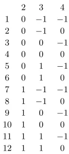
When there are five locations, there are 12 matrices describing restricted strategies resulting in 144 strategy pairs. The fol-lowing matrix describes these strategies. The first column is a number used to name the strategy. The action of the strategy at location 2,3,4 are given in the columns marked 2,3,4 respec-tively. For example, Strategy 6 is that of staying in place at location 2 moving to 4 from location 3 and staying in place at
location 4.
2 3 4
1 0 −1 −1
2 0 −1 0
3 0 0 −1
4 0 0 0
5 0 1 −1
6 0 1 0
7 1 −1 −1
8 1 −1 0
9 1 0 −1
10 1 0 0
11 1 1 −1
12 1 1 0
Of the 144 possible values ofbi97 result in values that are
dom-inated by other values so there are 47 non domdom-inated strategy pairs. We have listed below the 47 non dominated strategy pairs using the designations described in the matrix. The first number is the strategy used by I, the second by II and the third column is the resulting value ofb1.
1 8 p5,4+p4,2+p3,1+p2,3+p2,1+p1,3
1 10 p5,4+p4,3+p4,2+p3,1+p2,1
1 12 p5,4+p5,3+p4,2+p3,1+p2,1
2 2 p5,4+p4,5+p3,2+p3,1+p2,3+p2,1+p1,3+p1,2
2 6 p5,4+p5,3+p4,5+p4,3+p3,2+p3,1+p2,1+p1,2
3 7 p4,2+p3,4+p3,2+p2,3+p2,1+p1,3
3 8 p5,4+p4,2+p3,2+p2,3+p2,1+p1,3
3 9 p4,3+p4,2+p3,4+p3,2+p2,1
3 10 p5,4+p4,3+p4,2+p3,2+p2,1
3 11 p5,3+p4,2+p3,4+p3,2+p2,1
3 12 p5,4+p5,3+p4,2+p3,2+p2,1
4 7 p4,5+p3,4+p3,2+p2,3+p2,1+p1,3
4 11 p5,3+p4,5+p4,3+p3,4+p3,2+p2,1
5 8 p5,4+p4,2+p3,5+p3,4+p2,3+p2,1+p1,3
5 10 p5,4+p4,3+p4,2+p3,5+p3,4+p2,1
5 12 p5,4+p5,3+p4,2+p3,5+p3,4+p2,1
6 2 p5,4+p4,5+p3,5+p3,4+p2,3+p2,1+p1,3+p1,2
6 6 p5,4+p5,3+p4,5+p4,3+p3,5+p3,4+p2,1+p1,2
7 3 p4,3+p3,2+p3,1+p2,4+p2,3+p1,2
7 4 p5,4+p4,3+p3,2+p3,1+p2,3+p1,2
7 7 p4,2+p3,1+p2,4+p1,3
[image:4.612.405.476.85.242.2]7 10 p5,4+p4,3+p4,2+p3,1+p2,3
7 11 p5,3+p4,2+p3,1+p2,4
8 1 p4,5+p3,2+p3,1+p2,4+p1,3+p1,2
8 3 p4,5+p3,2+p3,1+p2,4+p2,3+p1,2
8 5 p5,3+p4,5+p4,3+p3,2+p3,1+p2,4+p1,2
9 3 p4,3+p3,4+p2,4+p2,3+p1,2
9 7 p4,2+p3,4+p3,2+p2,4+p1,3
9 9 p4,3+p4,2+p3,4+p3,2+p2,4+p2,3
9 10 p5,4+p4,3+p4,2+p3,2+p2,3
9 11 p5,3+p4,2+p3,4+p3,2+p2,4
10 1 p4,5+p3,4+p2,4+p1,3+p1,2
10 3 p4,5+p3,4+p2,4+p2,3+p1,2
10 5 p5,3+p4,5+p4,3+p3,4+p2,4+p1,2
10 7 p4,5+p3,4+p3,2+p2,4+p1,3
10 9 p4,5+p3,4+p3,2+p2,4+p2,3
10 11 p5,3+p4,5+p4,3+p3,4+p3,2+p2,4
11 3 p4,3+p3,5+p2,4+p2,3+p1,2
11 4 p5,4+p4,3+p3,5+p3,4+p2,3+p1,2
11 7 p4,2+p3,5+p2,4+p1,3
11 9 p4,3+p4,2+p3,5+p2,4+p2,3
11 10 p5,4+p4,3+p4,2+p3,5+p3,4+p2,3
11 11 p5,3+p4,2+p3,5+p2,4
12 1 p4,5+p3,5+p2,4+p1,3+p1,2
12 3 p4,5+p3,5+p2,4+p2,3+p1,2
12 5 p5,3+p4,5+p4,3+p3,5+p2,4+p1,2
Example 11 The most obvious situation occurs when both players begin at a location with equal and independent proba-bilities so that for each i, j, pi,j = 251. Any strategy in which
there is a maximal number of terms in the third column will then be optimal. These are (2,2),(2,6),(6,2),(6,6), having 8 terms. Each of these strategies will give an expected time of
8
25 + 2 1− 8 25−
5 25
= 3225. A similar situation is when both players are placed with equal probability at pairs of different lo-cations. The same strategy pairs are optimal and the expected time is then 8
20+ 2 1− 8 20
=8 5.
References
[1] S. Alpern and S. Gal, The theory of search games and ren-dezvous, International Series in Operations Research and Management Sciences, Kluwer, Boston, 2002.
[2] E. J. Anderson, R. R. Weber, ”The rendezvous problem on discrete locations”,Journal of Applied Probability28(1990) 335-340.
[3] V. J. Baston, ”Two rendezvous problems on the line”, Naval Research Logistics46 (1999) 335-340.
[4] Ruckle, W. H., ”Rendez-vous Search on a Rectangular Lat-tice”,Naval Research Logistics54: 492-496, 2007