Manipulating Large Corpora for Text Classification

Manipulating Large Corpora for Text Classification

Fumiyo Fukumoto and Yoshimi Suzuki

Department of Computer Science and Media Engineering, Yamanashi University

4-3-11 Takeda, Kofu 400-8511 Japan

[email protected] [email protected]

Abstract

In this paper, we address the problem of dealing with a large collection of data and propose a method for text classifi-cation which manipulates data using two well-known machine learning techniques, Naive Bayes(NB) and Support Vector Ma-chines(SVMs). NB is based on the as-sumption of word independence in a text, which makes the computation of it far more efficient. SVMs, on the other hand, have the potential to handle large feature spaces, which makes it possible to pro-duce better performance. The training data for SVMs are extracted using NB classifiers according to the category hier-archies, which makes it possible to reduce the amount of computation necessary for classification without sacrificing accuracy.

1 Introduction

As the volume of online documents has drastically increased, text classification has become more im-portant, and a growing number of statistical and ma-chine learning techniques have been applied to the task(Lewis, 1992), (Yang and Wilbur, 1995), (Baker and McCallum, 1998), (Lam and Ho, 1998), (Mc-Callum, 1999), (Dumais and Chen, 2000). Most of them use the Reuters-21578 articles1 in the

evalu-1

The Reuters-21578, distribution 1.0, is comprised of 21,578 documents, representing what remains of the original Reuters-22173 corpus after the elimination of 595 duplicates by Steve Lynch and David Lewis in 1996.

ations of their methods, since the corpus has be-come a benchmark, and their results are thus eas-ily compared with other results. It is generally agreed that these methods using statistical and ma-chine learning techniques are effective for classifi-cation task, since most of them showed significant improvement (the performance over 0.85 F1 score) for Reuters-21578(Joachims, 1998), (Dumais et al., 1998), (Yang and Liu, 1999).

and Chen, 2000).

The other is to use methods which are learning algorithms that construct a set of classifiers and then classify new data by taking a (weighted) vote of their predictions(Dietterich, 2000). One of the methods for constructing ensembles manipu-lates the training examples to generate multiple hy-potheses. The most straightforward way is called

. It presents the learning algorithm with a training set that consists of a sample of

examples drawn randomly with replacement from the original training set. The second method is to construct the training sets by leaving out disjoint subsets of the training data. The third is illustrated by the AD-ABOOST algorithm(Freund and Schapire, 1996). Dietterich has compared these methods(Dietterich, 2000). He reported that in low-noise data, AD-ABOOST performs well, while in high-noise cases, it yields overfitting because ADABOOST puts a large amount of weight on the mislabeled examples. Bagging works well on both the noisy and the noise-free data because it focuses on the statistical prob-lem which arises when the amount of training data available is too small, and noise increases this sta-tistical problem. However, it is not clear whether ‘works well’ means that it exponentially reduces the amount of computation necessary for classification, while sacrificing only a small amount of accuracy, or whether it is statistically significantly better than other methods.

In this paper, we address the problem of dealing with a large collection of data and report on an em-pirical study for text classification which manipu-lates data using two well-known machine learning techniques, Naive Bayes(NB) and Support Vector Machines(SVMs). NB probabilistic classifiers are based on the assumption of word independence in a text which makes the computation of the NB classi-fiers far more efficient. SVMs, on the other hand, have the potential to handle large feature spaces, since SVMs use overfitting protection which does not necessarily depend on the number of features, and thus makes it possible to produce better perfor-mance. The basic idea of our approach is quite sim-ple: We solve simple classification problems using NB and more complex and difficult problems using SVMs. As in previous research, we use category hierarchies. We use all the training data for NB.

The training data for SVMs, on the other hand, is extracted using NB classifiers. The training data is learned by NB using cross-validation according to the hierarchical structure of categories, and only the documents which could not classify correctly by NB classifiers in each category level are extracted as the training data of SVMs.

The rest of the paper is organized as follows. The next section provides the basic framework of NB and SVMs. We then describe our classification method. Finally, we report some experiments using 279,303 documents in the Reuters 1996 corpus with a discus-sion of evaluation.

2 Classifiers

2.1 NB

Naive Bayes(NB) probabilistic classifiers are com-monly studied in machine learning(Mitchell, 1996). The basic idea in NB approaches is to use the joint probabilities of words and categories to estimate the probabilities of categories given a document. The NB assumption is that all the words in a text are conditionally independent given the value of a clas-sification variable. There are several versions of the NB classifiers. Recent studies on a Naive Bayes classifier which is proposed by McCallum et. al. reported high performance over some other com-monly used versions of NB on several data collec-tions(McCallum et al., 1998). We use the model of NB by McCallum et. al. which is shown in formula (1).

! " #%$'&

( )"#*$+-,.0/, 1243

(5

.

/6 7 "#*$

,89,

:

243 (

:

)"#*$+ ,.;/<, 123

(5

.

/(6 7

:

"#%$

=?>@A9

(5B9C "#*$D& EF ,GH,

243I

(5 B J $( C $

LKM

F

,N@,

O

23 ,GH,

243 I (5

O

J$P(QR$

P( S" #*$D&

,GH,

243

( $0T

UV

(1)

WXYW

refers to the number of vocabularies,

WZ[W

de-notes the number of labeled training documents, and

W\]W

shows the number of categories.

W^)_`W

denotes document length. =ba

document , where the subscript of=

, indicates an index into the vocabulary. e[f

=hg;i ^ _;j

denotes the number of times word= g

occurs in document

^S_

, and

k

flm W^ _nj

is defined byk flm

W^ _ojqpsr

0,1t .

2.2 SVMs

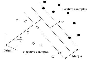
SVMs are introduced by Vapnik(Vapnik, 1995) for solving two-class pattern recognition problems. It is defined over a vector space where the problem is to find a decision surface(classifier) that ‘best’ sep-arates a set of positive examples from a set of nega-tive examples by introducing the maximum ‘margin’ between two sets. The margin is defined by the dis-tance from the hyperplane to the nearest of the pos-itive and negative examples. The decision surface produced by SVMs for linearly separable space is a hyperplane which can be written asuwvx +

= 0 (x ,

u

pzyh{

, p|y

), wherex is an arbitrary data point,

andu = ( =~}

,vLvv,

=

{ ) and

are learned from a train-ing set of linearly separable data. Figure 1 shows an example of a simple two-dimensional problem that is linearly separable2.

Margin Origin w w b − Positive examples Negative examples

Figure 1: The decision surface of a linear SVMs

In the linearly separable case maximizing the margin can be expressed as an optimization problem:

|€‚S€‚ƒ„€J…‡†ˆŠ‰ ‹ 243Œ F 3  ‹ ‚Ž 243Œ Œ <%Lo‘S’‘ (2) s.tˆ ‹ 243 Œ

“ &•”—– €˜ˆ

Œ ™ ” š & › 243Œ ‚‘S (3) wherex _ = (œ _ }

,vLvv,œ

_

{ ) is the

-th training example and

_

is a label corresponding the

-th training ex-ample. In formula (3), each element of w,=

d

(1ž

2

We focused on linear hypotheses in this work, while SVMs can handle nonlinear hypotheses usingŸ

† 7†¡

functions.

cž

) corresponds to each word in the training ex-amples, and the larger value of=

d¢ £ _)¤ _  _ œ _(d is, the more the word=

d

features positive examples. We note that SVMs are basically introduced for solving binary classification, while text classifica-tion is a multi-class, multi-label classificaclassifica-tion prob-lem. Several methods using SVMs which were in-tended for multi-class, multi-label data have been proposed(Weston and Watkins, 1998). We use¥

-LHL ¦§ -§>@ -¨ §

version of the SVMs model in the work. A time complexity of SVMs is known as ¥©f ‚ª j„« ¥bf ­¬ j , where

is the number of train-ing data. We consider a time complexity of ¥

¦ -LHL ¦§ -§>@ -¨ § method. Let

be the number of training data with c categories. The average

size of the training data per category is

£ d . Let also cR®¯v4°©f ® j

be the time needed to train all cat-egories, where °±f

®

j

represents the time for learn-ing one binary classifier uslearn-ing

® training data, and c ® is the number of binary classifier. The time for

learning one binary classifier,°©f

®

j

is represented as

°©f ® j²¢ \ v ® ¬ , where \

is a constant.¥ -˜L § -§>@ -¨ §

method is thus done in time

\

c

0¬

.

3 System Design

3.1 Hierarchical classification

A well-known technique for classifying a large, het-erogeneous collection such as web content is to use category hierarchies. Following the approaches of Koller and Sahami(Koller and Sahami, 1997), and Dumais’s(Dumais and Chen, 2000), we employ a hi-erarchy by learning separate classifiers at each in-ternal node of the tree, and then labeling a docu-ment using these classifiers to greedily select sub-branches until a leaf is reached.

3.2 Manipulating training data

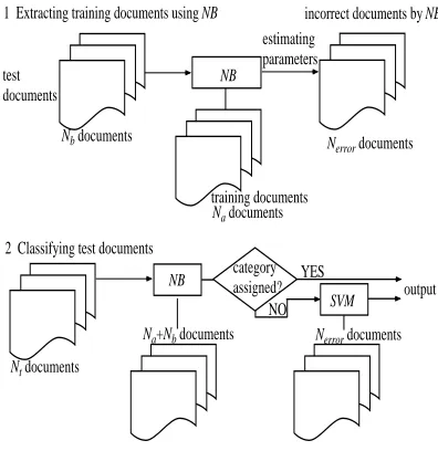
cat-egory level(Lewis and Ringuette, 1994), (Koller and Sahami, 1997). SVMs, on the other hand, have the potential to handle more complex problems without sacrificing accuracy, even though the computation of the SVM classifiers is far less efficient than NB. We thus use NB for simple classification problems and SVMs for more complex data, i.e., the data which cannot be classified correctly by NB classifiers. We use ten-fold cross validation: All of the training data were randomly shuffled and divided into ten equal folds. Nine folds were used to train the NB clas-sifiers while the remaining fold(held-out test data) was used to evaluate the accuracy of the classifica-tion. For each category level, we apply the following procedures. Leteb³ be the total number of nine folds

training documents, ande•´ be the number of the

re-maining fold in each class level. Figure 2 illustrates the flow of our system.

1 Extracting training documents using NB

test documents

Nb documents

NB

estimating parameters

incorrect documents by NB

Nerror documents

training documents

2 Classifying test documents

Nt documents

NB

SVM output

Na+Nb documents Nerror documents

Na documents

category assigned?

NO YES

Figure 2: Flow of our system

1. Extracting training data using NB

1-1 NB is applied to thee~³ documents, and

clas-sifiers for each category are induced. They are evaluated using the held-out test data, the e ´

documents.

1-2 This process is repeated ten times so that each fold serves as the source of the test data once. The threshold, the probability value which pro-duces the most accurate classifier through ten runs, is selected.

1-3 The held-out test data which could not be clas-sified correctly by NB classifiers with the opti-mal parameters are extracted (e-µn¶n¶C·C¶ in Figure

2). They are used to train SVMs.

The procedure is applied to each category level.

2. Classifying test data

2-1 We use all the training data, e~³ +e¸´ , to train

NB classifiers and the data which is produced by procedure 1-3 to train SVMs.

2-2 NB classifiers are applied to the test data. The test data is judged to be the category l whose

probability is larger than the threshold which is obtained by 1-2.

2-3 If the test data is not assigned to any one of the categories, the test data is classified by SVMs classifiers. The test data is judged to be the cat-egoryl whose distance

}

¹¹`º

»

¹¼¹ is larger than zero.

We employ the hierarchy by learning separate classi-fiers at each internal node of the tree and then assign categories to a document by using these classifiers to greedily select sub-branches until a leaf is reached.

4 Evaluation

4.1 Data and Evaluation Methodology

We evaluated the method using the 1996 Reuters corpus recently made available. The corpus from 20th Aug. to 31st Dec. consists of 279,303 doc-uments. These documents are organized into 126 categories with a four level hierarchy. We selected 102 categories which have at least one document in the training set and the test set. The number of cate-gories in each level is 25 top level, 33 second level, 43 third level, and 1 fourth level, respectively. Table 1 shows the number of documents in each top level category.

Category name Training Test

Corporate/Industrial 69,975 56,100

Economics 22,214 18,694

Government/social 45,618 36,923

Crime 6,248 4,865

Defence 1,646 1,408

International relations 7,523 6,278

Disasters 1,644 1,383

Arts 771 602

Environment 1,170 876

Fashion 71 14

Health 1,232 961

Labour issues 3,314 2,827

Obituaries 123 124

Human interest 479 418

Domestic politics 11,528 9,022

Biographies 1,115 1,041

Religion 618 418

Science and technology 359 410

Sports 5,807 4,998

Travel and tourism 149 142

War 7,064 5,228

Elections 3,070 1,944

Weather 784 474

Welfare 359 260

Markets 34,901 28,484

Total 227,782 183,894

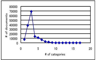
Table 1: Top level categories

in the training set. The number of categories per document is 3.2 on average.

Figure 3: Category distribution in Reuters 1996

We use ten-fold cross validation for learning NB parameters. For evaluating the effectiveness of cate-gory assignments, we use the standard recall, preci-sion, and ½¿¾ measures. Recall denotes the ratio of

correct assignments by the system divided by the to-tal number of correct assignments. Precision is the ratio of correct assignments by the system divided by the total number of the system’s assignments.

The½b¾ measure which combines recall (

A

) and pre-cision (À ) with an equal weight is½¿¾f

Ai

À

jq¢

ª

¶CÁ ¶Â)Á . 4.2 Results and Discussion

The result is shown in Table 2.

category Performance

miR miP miF1

NB all 0.684 0.419 0.519

parts 0.565 0.523 0.543

SVMs all 0.318 0.258 0.285

parts 0.795 0.554 0.653

Manipulating all 0.703 0.704 0.704

data parts 0.720 0.692 0.700

Table 2: Categorization accuracy

‘NB’, ‘SVMs’, and ‘Manipulating data’ denotes the result using Naive Bayes, SVMs classifiers, and our method, respectively. ‘miR’, ‘miP’, and ‘miF1’ refers to the micro-averaged recall, precision, and F1, respectively. ‘all’ in Table 2 shows the results of all 102 categories. The micro-averaged F1 score of our method in ‘all’ (0.704) is higher than the NB (0.519) and SVMs scores (0.285). We note that the F1 score of SVMs (0.285) is significantly lower than other models. This is because we could not obtain a classifier to judge the category ‘corporate/industrial’ in the top level within 10 days using a standard 2.4 GHz Pentium IV PC with 1,500 MB of RAM. We thus eliminated the category and its child categories from the 102 categories. The number of the remain-ing categories in each level is 24 top, 14 second, 29 third, and 1 fourth level. ‘Parts’ in Table 2 de-notes the results. There is no significant difference between ‘all’ and ‘parts’ in our method, as the F1 score of ‘all’ was 0.704 and ‘parts’ was 0.700. The F1 of our method in ‘parts’ is also higher than the NB and SVMs scores.

Table 3 denotes the amount of training data used to train NB and SVMs in our method and test data judged by each classifier. We can see that our method makes the computation of the SVMs more efficient, since the data trained by SVMs is only 23,243 from 150,939 documents.

cate-Manipulating # of selected documents _{miR miP miF1}

data training test

NB 150,939 76,650 0.798 0.674 0.730

SVMs 23,243 43,592 0.789 0.588 0.674

Total performance 0.703 0.704 0.704

Table 3: # of selected documents and categorization accuracy

Top level(25 categories)

training miR miP miF1

NB 147,576 0.877 0.573 0.693

SVMs 147,576 0.358 0.325 0.341

Manipulating _{22,528 0.836 0.679 0.715}

data

Second level(33 categories)

training miR miP miF1

NB 129,130 0.559 0.529 0.543

SVMs 129,130 0.327 0.302 0.314

Manipulating _{17,667 0.833 0.478 0.608}

data

Third level(43 categories)

training miR miP miF1

NB 92,320 0.609 0.383 0.471

SVMs 92,320 0.318 0.258 0.258

Manipulating _{12,482 0.820 0.481 0.606}

data

Fourth level(1 category)

training miR miP miF1

NB 150,939 0.397 0.184 0.251

SVMs 150,939 0.318 0.258 0.258

Manipulating _{150,939 0.297 0.241 0.265}

data

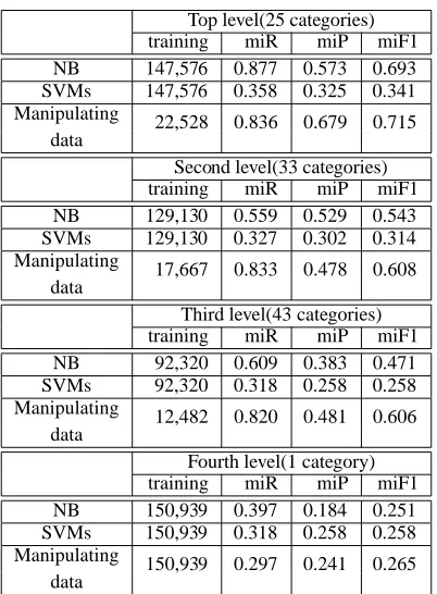
Table 4: Categorization accuracy by category level

gories is 0.693, 0.341, and 0.715, respectively. Clas-sifying large corpora with similar categories is a difficult task, so we did not expect to have excep-tionally high accuracy like Reuters-21578 (0.85 F1 score). Performance on the original training set us-ing SVMs is 0.285 and usus-ing NB is 0.519, so this is a difficult learning task and generalization to the test set is quite reasonable.

There is no significant difference between the overall F1 value of the second(0.608) and third level categories(0.606) in our method, while the accuracy of the other methods drops when classifiers select sub-branches, in third level categories. As Dumais et. al. mentioned, the results of our experiment show that performance varies widely across cate-gories. The highest F1 score is 0.864 (‘Commodity markets’ category), and the lowest is 0.284

(‘Eco-nomic performance’ category).

The overall F1 values obtained by three methods for the fourth level category (‘Annual result’) are low. This is because there is only one category in the level, and we thus used all of the training data, 150,939 documents, to learn models.

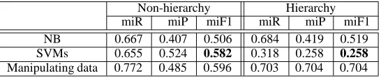
The contribution of the hierarchical structure is best explained by looking at the results with and without category hierarchies, as illustrated in Table 5. It is interesting to note that the results of both NB and our method clearly demonstrate that incor-porating category hierarchies into the classification method improves performance, whereas hierarchies degraded the performance of SVMs. This shows that the separation of one top level category(C) from the set of the other 24 top level categories is more dif-ficult than separating C from the set of all the other 101 categories in SVMs.

Table 6 illustrates sample words which have the highest weighted value calculated using formula (3). Recall that in SVMs each value of word=

d

(1 ž

cVž

) is calculated using formula (3), and the larger value of =

d

is, the more the word =

d

Non-hierarchy Hierarchy

miR miP miF1 miR miP miF1

NB 0.667 0.407 0.506 0.684 0.419 0.519

SVMs 0.655 0.524 0.582 0.318 0.258 0.258

Manipulating data 0.772 0.485 0.596 0.703 0.704 0.704

Table 5: Non-hierarchical v.s. Hierarchical categorization accuracy

humans.

Economics

Hierarchy access, Ford, Japan, Internet,

econ-omy, year, sale, service, month, market

Non-hierarchy economic, economy, industry, ltd.,

company, Hollywood, business,

service, Internet, access

Table 6: Sample words

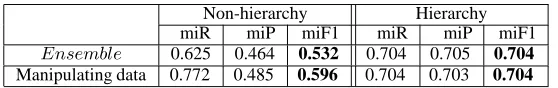
Finally, we compare our results with a well-known technique, ¦

strategies. In the ex-periment using ensemble, we divided a training set into ten folds for each category level. Once the indi-vidual classifiers are trained by SVMs they are used to classify test data. Each classifier votes and the test data is assigned to the category that receives more than 6 votes3. The result is illustrated in Table 7. In Table 7, ‘Non-hierarchy’ and ‘Hierarchy’ denotes the result of the 102 categories treated as a flat non-hierarchical problem, and the result using hierarchi-cal structure, respectively. We can find that the re-sult of ¦%

with hierarchy(0.704 F1) outper-forms the result with non-hierarchy(0.532 F1). A necessary and sufficient condition for an ensemble of classifiers to be more accurate than any of its in-dividual members is if the classifiers are

l‡loÃ

A

§

and

^

ÅÄ A9

(Hansen and Salamon, 1990). An ac-curate classifier is one that has an error rate bet-ter than random guessing on new test data. Two classifiers are diverse if they make different errors on new data points. Given our result, it may be safely said, at least regarding the Reuters 1996 cor-pus, that hierarchical structure is more effective for constructing ensembles, i.e., an ensemble of clas-sifiers which are constructed by the training data with fewer than 30 categories in each level is more

lloÃ

A

§

and

^

ÅÄ A9

. Table 7 shows that our

method and ¦%

perform equally (0.704 F1 3

6 votes was the best results among 10 different voting schemes in the experiment.

score) when we use hierarchical structure. How-ever, the computation of the former is far more ef-ficient than the latter. Furthermore, we see that our method (0.596 F1 score) slightly outperforms

¦

(0.532 F1 score) when the 102 categories are treated as a flat non-hierarchical problem.

5 Conclusions

We have reported an approach to text classifica-tion which manipulates large corpora using NB and SVMs. Our main conclusions are:

Æ

Our method outperforms the baselines, since the micro-averaged ½b¾ score of our method

was 0.704 and the baselines were 0.519 for NB and 0.285 for SVMs.

Æ

As shown in previous researches, hierarchical structure is effective for classification, since the result of our method using hierarchical struc-ture led to as much as a 10.8% reduction in er-ror rates, and up to 1.3% with NB.

Æ

There is no significant difference between the F1 scores of our method and the ¦

method with hierarchical structure. However, the computation of our method is more efficient

than the¦

method in the experiment.

Future work includes (i) extracting features which discriminate between categories within the same top-level category, (ii) investigating other machine learning techniques to obtain further advantages in efficiency in the manipulating data approach, and (iii) evaluating the manipulating data approach us-ing automatically generatus-ing hierarchies(Sanderson and Croft, 1999).

Acknowledgments

Non-hierarchy Hierarchy

miR miP miF1 miR miP miF1

ÇȁHɆƒ„Êo¡­†

0.625 0.464 0.532 0.704 0.705 0.704

Manipulating data 0.772 0.485 0.596 0.704 0.703 0.704

Table 7: Performance ofË v.s. Manipulating data

and the anonymous reviewers for their helpful sug-gestions. We also would like to express many thanks to the Research and Standards Group of Reuters who provided us the corpora.

References

L. D. Baker and A. K. McCallum. 1998. Distributional Clustering of Words for Text Classification. In Proc.

of the 22nd Annual International ACM SIGIR Confer-ence on Research and Development in Information Re-trieval, pages 96–103.

T. G. Dietterich. 2000. Ensemble Methods in Machine Learning. In Proc. of the 1st International Workshop

on Multiple Classifier Systems.

S. Dumais and H. Chen. 2000. Hierarchical Classifi-cation of Web Content. In Proc. of the 23rd Annual

International ACM SIGIR Conference on Research and Development in Information Retrieval, pages 256–

263.

S. Dumais, J. Platt, D. Heckerman, and M. Sahami. 1998. Inductive Learning Algorithm and Representations for Text Categorization. In Proc. of ACM-CIKM98, pages 148–155.

Y. Freund and R. E. Schapire. 1996. Experiments with a New Boosting Algorithm. In Proc. of the 13th

In-ternational Conference on Machine Learning, pages

148–156.

L. Hansen and P. Salamon. 1990. Neural Network En-sembles. IEEETrans. Pattern Analysis and Machine

Intell., 12:993–1001.

T. Joachims. 1998. Text Categorization with Support Vector Machines: Learning with Many Relevant Fea-tures. In Proc. of the Conference on Machine

Learn-ing, pages 96–103.

D. Koller and M. Sahami. 1997. Hierarchically Classi-fying Documents using Very Few Words. In Proc. of

the 14th International Conference on Machine Learn-ing, pages 170–178.

W. Lam and C. Y. Ho. 1998. Using a Generalized In-stance Set for Automatic Text Categorization. In Proc.

of the 21st Annual International ACM SIGIR Confer-ence on Research and Development in Information Re-trieval, pages 81–89.

D. D. Lewis and M. Ringuette. 1994. Comparison of Two Learning Algorithms for Text Categorization. In Proc. of the 3rd Annual Symposium on Document

analysis and Information Retrieval.

D. D. Lewis. 1992. An Evaluation of Phrasal and Clus-tered Representations on a Text Categorization Task. In Proc. of the 15th Annual International ACM SIGIR

Conference on Research and Development in Informa-tion Retrieval, pages 37–50.

A. K. McCallum, R. Rosenfeld, T. Mitchell, and A. Ng. 1998. Improving Text Classification by Shrinkage in a Hierarchy of Classes. In Proc. of the 15th

Interna-tional Conference on Machine Learning, pages 359–

367.

A. K. McCallum. 1999. Multi-Label Text Classification with a Mixture Model Trained by EM. In Revised

ver-sion of paper appearing in AAAI’99 Workshop on Text Learning.

T. Mitchell. 1996. Machine Learning. McGraw Hill.

D. Mladenic and M. Grobelnik. 1998. Feature Selection for Classification based on Text Hierarchy. In Proc. of

the Workshop on Learning from Text and the Web.

M. Sanderson and B. Croft. 1999. Deriving Concept Hi-erarchies from Text. In Proc. of the 22nd Annual

Inter-national ACM SIGIR Conference on Research and De-velopment in Information Retrieval, pages 206–213.

H. Schmid. 1995. Improvements in Part-of-Speech Tag-ging with an Application to German. In Proc. of the

EACL SIGDAT Workshop.

V. Vapnik. 1995. The Nature of Statistical Learning

The-ory. Springer.

J. Weston and C. Watkins. 1998. Multi-Class Support Vector Machines. In Technical Report

CSD-TR-98-04.

Y. Yang and X. Liu. 1999. A Re-Examination of Text Categorization Methods. In Proc. of the 22nd Annual

International ACM SIGIR Conference on Research and Development in Information Retrieval, pages 42–

49.

Y. Yang and W. J. Wilbur. 1995. Using Corpus Statistics to Remove Redundant Words in Text Categorization.