Swarm Intelligence in the Optimization of
Concurrent Service Systems
Tad Gonsalves and Kiyoshi Itoh, Members, IEEE
Abstract— Concurrent service systems are modeled using the Generalized Stochastic Petri Nets (GSPN) to account for the multiple asynchronous activities within the system. The simulated operation of the GSPN modeled system is then optimized using the Particle Swarm Optimization (PSO) meta-heuristic algorithm. The objective function consists of the service costs and the waiting costs. Service cost is the cost of hiring service-providing professionals, while waiting cost is the estimate of the loss to business as some customers might not be willing to wait for the service and may decide to go to the competing organizations. The optimization is subject to the management and to the customer satisfaction constraints. The tailor-made PSO is found to converge rapidly yielding optimum results for the operation of a practical concurrent service system.
Index Terms—Meta-heuristics, Optimization, Particle Swarm Optimization, Swarm Intelligence.
I. INTRODUCTION A. Swarm Intelligence
The Particle Swarm Optimization (PSO) is based on the Swarm Intelligence Paradigm of Evolutionary Computation. The algorithm is inspired by the social behavior of birds and fish swarming together to search for food [31], [32]. PSO has been successfully applied to solving optimization problems in diverse disciplines. Compared to other evolutionary computational algorithms, PSO has many desirable characteristics. PSO is easy to implement, can achieve high-quality solutions quickly, and has the flexibility in balancing global and local exploration.
The population-based PSO conducts a search using a population (swarm) of individuals called particles. The performance of each particle is measured according to a predefined fitness function. Particles are assumed to “fly” over the search space in order to find promising regions of the landscape. Each particle is treated as a point in a d-dimensional space which adjusts its own “flying” according to its flying experience as well as the flying experience of the other companion particles. By making adjustments to the flying based on the local best (pbest) and the global best (gbest) found so far, the swarm as a whole converges to the optimum point, or at least to a near-optimal point, in the search space.
Manuscript received December 30, 2008. This work has been supported by the Open Research Center Project funds from “MEXT” of the Japanese Government (2007-20011).
T. Gonsalves is with the Department of Information & Communication Sciences, Sophia University, Tokyo, Japan (phone: 81-3-3238-4143; fax: 81-3-3238-3311; e-mail: t-gonsal@ sophia.ac.jp).
K. Itoh is with the Department of Information & Communication Sciences, Sophia University, Tokyo, Japan (e-mail: itohkiyo@ sophia.ac.jp).
Operational costs of service systems
A service system is a configuration of technology and organizational networks designed with the intention of providing service to the end users. Practical service systems include hospitals, banks, ticket-issuing and reservation offices, restaurants, ATM, etc. The managerial authorities are often pressed to drastically reduce the operational costs of active and fully functioning service systems, while the system designers are forced to design (new) service systems operating at minimal costs. Both these situations involve system optimization.
Any optimization problem involves the objective to be optimized and a set of constraints [1]. In this study, we seek to minimize the total cost (tangible and intangible) to the system. The total cost can be divided into two broad categories - cost associated with the incoming customers having to wait for the service (waiting cost) and that associated with the personnel (servers) engaged in providing service (service cost) [2]-[4]. Waiting cost is the estimate of the loss to business as some customers might not be willing to wait for the service and may decide to go to the competing organizations, while serving cost is mainly due to the salaries paid to employees.
Business enterprises and companies often mistakenly “throw” capacity at a problem by adding manpower or equipment to reduce the waiting costs. However, too much capacity decreases the profit margin by increasing the production and/or service costs [5]. The managerial staff, therefore, is required to balance the two costs and make a decision about the provision of an optimum level of service. In recent years, customer satisfaction has become a major issue in marketing research and a number of customer satisfaction measurement techniques have been proposed [6]-[8]. Increasing efforts have been made to analyze the causes of customer dissatisfaction and to suggest remedies [9], [10]. In queuing systems, nothing can be as detrimental to customer satisfaction as the experience of waiting for service. For customers, waiting is frustrating, demoralizing, agonizing, aggravating, annoying, time-consuming, and incredibly expensive [11]. Waiting has a negative impact on service quality evaluations [12], [13].
customers. Hence, we define the customer satisfaction constraint as fuzzy sets.
In this study, we use the restaurant service system as a practical illustration of the meta-heuristic optimization procedure. Being a concurrent system (independent and asynchronous activities are taking place simultaneously), it is modeled as a Generalized Stochastic Petri Net. The system operation is simulated through a discrete event simulator [17] and the functional aspects of the system are visually verified. The queuing statistics obtained from the simulation are used to compute the waiting costs. The objective function consisting of the service cost and the waiting cost is minimized with the rapidly converging PSO meta-heuristic, subject to the customer satisfaction fuzzy constraint.
B. Petri net model of service systems
Service systems are inherently concurrent with multiple asynchronous activities. The traditional methods developed for the analysis of sequential systems are found to be inadequate for the analysis of systems exhibiting concurrency and synchronization of independent, asynchronous activities [18]. Petri nets are found to be ideal tools to model distributed and concurrent systems [19]-[21]. The original Petri net (PN) is a directed bipartite graph with two types of nodes, called places (represented by circles) and transitions (represented by horizontal or vertical bars). Directed arcs connect places to transitions, and vice versa. Places may contain tokens (represented by black dots). Places represent the conditions to be met before the transitions can fire. A transition is said to be enabled if there is at least one token in each of its input places. An enabled transition can fire by removing a token from each input place and depositing a token in each output place [22], [23]. The transitions fire instantaneously, implying that events do not take any time. Since there is no concept of time duration in the classical PN, it is not complete enough for the study of systems performance. Several concepts of timed Petri nets have been proposed by assigning firing times to the transitions and/or places of Petri nets [24]-[29]. Timed PNs in which the firing time is deterministic (constant) are called D-nets, while those in which the firing time is stochastic are called M-nets. Time-nets with transitions containing both kinds of firing times are called Generalized Stochastic Petri Net (GSPN) [30].
Fig. 1. Client Server GSPN
In addition, the customer flow and the server roles are made explicit in our Petri net modeled concurrent business
systems. The server resides in the serve place (SP), while the customer resides in the customer place (CP) as shown in Fig. 1. The service at a transition T can begin only when there is at least one server in the SP and correspondingly at least one customer in the CP. Making the customer and the server workflows distinct gives a more realistic analysis of the system.
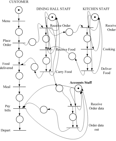
We use a GPSN to model concurrent business systems. A restaurant business system modeled as a client server GSPN is shown in Fig. 2.
[image:2.595.306.544.193.482.2]
Fig. 2. Petri net model of a restaurant
places provides the queuing statistics like the average queue length, the average queuing time and the maximum number of customers in the queues. Similarly, the data set associated with the server places provides the average server utilization. The simulation output data is then used to evaluate the objective function to be optimized.
II. FORMULATION OF OPTIMIZATION PROBLEM A. Objective Function
If Cw is the average waiting cost per customer per unit time
and Nw is the average number of customers waiting for
service, then the waiting cost per unit time at a given PN customer place is:
WC = NwCw (1)
The service cost in the service systems is the sum of the costs required to hire professionals to provide service to customers. If NS is the number of servers serving at a
transition and CS is the cost per server per unit time, then the
service cost at that transition per unit time is:
SC = NSCS (2)
The objective function (total cost) is given by:
f =
∑
Nwi Cwi + NSjCSj (3) =n
i1
∑
=m
1 j
[image:3.595.61.290.459.630.2]where, n is the number of waiting places and m is the number of server groups in the PN.
Fig. 3. Service cost and waiting cost in queuing systems
B. Management Constraints
Each service activity has an appropriate service time that is usually drawn from an exponential distribution. The service time constraints can be expressed as:
ST< ≤ ST ≤ ST> (4)
where, ST< and ST> are respectively the minimum and
maximum values of the service time at a given PN transition.
The capacity of the server represents the number of servers allotted to a given transition. If NS is the capacity of a
server, serving at a group of transitions, then the constraints are:
NS< ≤ NS ≤ NS> (5)
Similarly, the priority constraints of the servers with respect to a given transition are:
Pr< ≤ Pr ≤ Pr> (6)
where, Pr< and Pr> are respectively the minimum and the
maximum values of the servers with respect to a given PN transition.
C. Customer Satisfaction Constraints
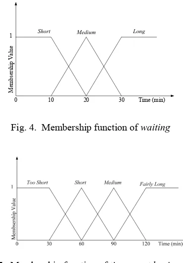
In service systems, customer satisfaction depends on the waiting as well as the service experience. In the restaurant system, if the waiting is too long, the customers are dissatisfied. On the other hand, if they are not allowed to enjoy their meal for a sufficiently long period to time, then they are dissatisfied, too. Consequently, customer satisfaction can be increased by decreasing the waiting time and by increasing the service time (meal time). In this section, we describe the fuzzy membership functions of the waiting and eating experiences.
The membership functions are defined in such a way that they appropriately reflect the changes in the degree of membership in each set, associated with changes in the crisp value [33]-[37]. Fig. 4 illustrates the membership functions for the fuzzy sets pertaining to the variable waiting. Here, the linguistic variables are Short, Medium and Long. Fig. 4 illustrates the membership functions for the variable time spent having meal. The linguistic variables are: Too Short, Short, Medium and Fairly Long.
Number of Servers
Waiting Cost Service Cost Total Cost
Cost
Membs
ers
hi
p V
alue
10 20 30 Time (min)
Short Medium Long
1
[image:3.595.335.520.491.757.2]0
Fig. 4. Membership function of waiting
[image:3.595.343.525.647.743.2]in waiting) and those for service (time spent in having meal) to produce a single fuzzy output.
Table I Fuzzy rules matrix
[image:4.595.66.274.271.384.2]The final customer satisfaction membership function values obtained by the combination of the above rules are shown in Fig. 6.
Fig. 6. Membership function of customer satisfaction Defuzzification is the process by which the output fuzzy variables are converted into a unique (crisp) value. The max method and the centroid methods are well-known methods for obtaining the crisp value from the superposition of the fuzzy membership functions. In our study, the final decision on the waiting and service experience is arrived at by using the centroid method (Equation 7). In the restaurant service system, at least 50% fairly good and 50% good customer satisfaction is desirable. This corresponds to 0.625 crisp value on the decision index as shown in Fig. 6.
FD =
∑
∑
μ
μD (7)
III. PARTICLE SWARM OPTIMIZATION
The Particle Swarm Optimization (PSO) algorithm imitates the information sharing process of a flock of birds searching for food. The population-based PSO conducts a search using a population of individuals. The individual in the population is called the particle and the population is called the swarm. The performance of each particle is measured according to a predefined fitness function. During the search, each particle records its local best (pbest), and the swarm records the global best (gbest) found so far. In every iteration, the particles move taking into consideration their previous pbest as well as the swarm gbest. The process is repeated till the convergence of the swarm occurs.
The notations used in PSO are as follows: The ith particle of
the swarm in iteration t is represented by the d-dimensional
vector, xi(t) = (xi1, xi2,…, xid). Each particle also has a position
change known as velocity, which for the ith particle in
iteration t is vi(t) = (vi1, vi2,…, vid). The best previous position
(the position with the best fitness value) of the ith particle is p
i
(t-1) = (pi1, pi2,…, pid). The best particle in the swarm, i.e., the
particle with the smallest function value found in all the previous iterations, is denoted by the index g. In a given iteration t, the velocity and position of each particle is updated using the following equations:
Short me dium Long
T oo Short poor poor v ery poor
Short fairly good poor v ery poor
Me dium good fairly good poor
Fairly Long very good good fairly good
D
I
N
I
N
G
W A I T I N G
vi(t) = wvi(t-1) + c1r1(pi(t-1) - xi(t-1))
+ c2r2(pg(t-1) - xi (t-1)) (8)
and
xi(t) = xi(t-1) + vi(t) (9)
where, i =1, 2,…, NP; t = 1, 2,…,T. NP is the size of the swarm, and T is the iteration limit; c1 and c2 are constants; r1
and r2 are random numbers between 0 and 1; w is the inertia
weight that controls the impact of the previous history of the velocities on the current velocity, influencing the trade-off between the global and local experiences. A large inertia weight facilitates global exploration (searching new areas), while a small one tends to facilitate local exploration (fine-tuning the current search area). Equation 8 is used to compute a particle’s new velocity, based on its previous velocity and the distances from its current position to its local best and to the global best positions. The new velocity is then used to compute the particle’s new position (Equation 9). In our application, the decision variables (Table 1) are the particles’ “positions” and “velocities”. Initially, a group (population) of particles is randomly generated. Their fitness function f (Equation 3) is evaluated on simulating the system operation. The algorithm is iterated for a fixed number of iterations. The particles’ velocities and positions are updated using Equations 8 and 9, in every iteration. The lowest value of the fitness function attained by a particle in all the iterations is its pbest, while that of the entire population is the gbest. The latter is the optimum value of the objective function.
IV. RESULTS OF PSO OPTIMIZATION
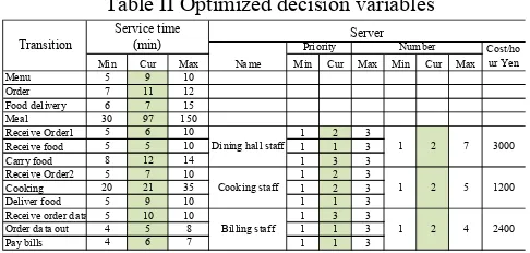
The current (cur) optimized values of the decision variables (service time, number of staff members or severs and their priority at each activity) are shown in Table II. These values are bounded between the given minimum (min) and the maximum (max) values. The restaurant operation is simulated for six hours for an average inter-arrival time of 15 minutes. The minimized total cost (sum of the waiting and the serving cost) is found to be 4358,457 yen.
Table II Optimized decision variables
Min Cur Max Name Min Cur Max Min Cur Max
Menu 5 9 10
Order 7 11 12
Food delivery 6 7 15
Meal 30 97 150
Receive Order1 5 6 10 1 2 3
Receive food 5 5 10 1 1 3
Carry food 8 12 14 1 3 3
Receive Order2 5 7 10 1 2 3
Cooking 20 21 35 1 2 3
Deliver food 5 9 10 1 1 3
Receive order data 5 10 10 1 3 3
Order data out 4 5 8 1 1 3
Pay bills 4 6 7 1 1 3
3000
Server
Priority Number Cost/ho
ur Yen
2400
Cooking staff 1 2 5 1200
Transition
Service time (min)
Billing sta 1 2 4
Dining hall staff 1 2 7
[image:4.595.303.546.644.760.2]V. CONCLUSION
In this paper, we have presented the application of the PSO meta-heuristic algorithm in the optimization of the operation of a practical service system, subject to the customer satisfaction constraint. The cost function is expressed as the sum of the service cost and the waiting cost. Service cost is due to hiring professionals or equipment to provide service to end users. Waiting cost emerges when customers are lost owing to unreasonable amount of waiting for service. Waiting can be reduced by increasing the number of personnel. However, increasing the number of personnel, results in a proportional increase in the service cost. The simulation optimization strategy finds the optimum balance between the service cost and the waiting cost. The optimization, however, is subject to the customer satisfaction constraint, which is defined as fuzzy sets quantifying the waiting as well as the service experiences of the customers. The simulation optimization strategy finds the optimum balance between the service cost and the waiting cost without violating the customer satisfaction constraint. PSO obtains the optimum results with rapid convergence even for a very large search space. An extension to this study would be multi-objective optimization.
REFERENCES
[1] C. Reeves, Genetic Algorithms, F. Glover and G. A. Kochenberger (eds.), Handbook of Metaheuristics, Kluwer Academic Publications, Boston, 2003.
[2] F. S. Hillier, Economic Models for Industrial Waiting Line Problems, Management Science, Vol. 10, No.1, 1963, pp. 119-130.
[3] D. R. Anderson, D. J. Sweeney and T. A. Williams, An Introduction to Management Science: Quantitative Approaches to Decision Making (10th ed.), Thomson South-Western, Ohio, 2003.
[4] Y. A. Ozcan, Quantitative Methods in Health Care Management: Techniques and Applications, Jossey-Bass/Wiley, San Francisco, 2005.
[5] K. V. Buxon and R. Gatland, (1995), “Simulating the effects of work-in-progress on customer satisfaction in a manufacturing environment”, C. Alexopolous, K. Kang, W. R. Lilegdon, and D. Goldman (eds.), Proceedings of the 1995 Winter Simulation Conference.
[6] L. Dube-Rioux, B.H.Schmitt, F. Leclerc, (1988), "Consumer’s reactions to waiting: when delays affect the perception of service quality", in Srull, T. (Eds), Advances in Consumer Research, Association for Consumer Research, Provo, UT, Vol. 16 pp.59-63. [7] K.L. Katz, B.M. Larson, and R.C. Larson, (1991), "Prescription for the
waiting-in-blues: entertain, enlighten, and engage", Sloan Management Review, Vol. 32 pp.44-53.
[8] V. S. Folkes, “Consumer Reactions to Product Failure: An
Attributional Approach”, The Journal of Consumer Research, Vol. 10, No. 4. (Mar., 1984), pp. 298-409.
[9] S. Taylor, (1995), "The effects of filled waiting time and service provider control over the delay on evaluations of service", Journal of the Academy of Marketing Science, Vol. 23 No.1, pp.38-48.. [10] V.S. Folkes, S. Koletsky, and J. L. Graham, (1987), “A field study of
causal inferences and consumer reaction: the view from the airport”, Journal of Consumer Behavior, Vol. 13 pp.534-9.
[11] D.H. Maister, (1985), “The psychology of waiting lines”, in Czepiel, J., Solomon, M.R., Surprenant, C.F. (Eds),The Service Encounter, Lexington Books, Lexington, MA, pp.113-23.
[12] S. Taylor, (1994), “Waiting for service: the relationship between delays and evaluation of service”, Journal of Marketing, Vol. 58 pp.56-69. [13] R. Scotland, (1991), “Customer service: a waiting game”, Marketing,
pp.1-3.
[14] L. A. Zadeh, ‘‘Fuzzy Sets”, Information and Control, Vol. 8, 1965, pp 338-359.
[15] H. Zimmermam, Fuzzy Sets, Decision Making, and Expert Systems, Kluwer Academic, Boston, 1987.
[16] T. Terano, K. Asai, and M. Sugeno, Fuzzy systems theory and its applications, Boston : Academic Press , 1992.
[17] G. S. Fishman, Principles of Discrete Event Simulation, John Wiley & Sons, New York, 1978.
[18] W.M. Zuberek, “D-timed Petri nets and modelling of timeouts and protocols”, Trans. of the Society for Computer Simulation, vol.4, no.4 (1988) 331-357.
[19] M. Ajmone-Marsan, G. Balbo, G. Conte, “A class of Generalized Stochastic Petri Nets for the performance evaluation of multiprocessor systems”, ACM Transactions on Computer Systems, Vol. 2, No. 2, May 1984, pp. 93-122.
[20] M.K. Molloy, “Performance analysis using stochastic Petri nets”, IEEE Trans. on Computers, vol.31, no.9, pp.913-917, 1982.
[21] J.L. Peterson, Petri net theory and the modeling of systems. Prentice-Hall, 1981.
[22] J.L. Peterson, 1977, “Petri Nets,” Computing Surveys, Vol. 9, No.3. [23] T. Murata, Petri nets - properties, analysis, and applications, Proc.
IEEE, vol.77, no.4, (1989)541-580.
[24] T. Agerwala, Putting Petri nets to work, IEEE Computer, vol.12, no.12 (1979) 85-94.
[25] C. V. Ramamoorthy and G. S. Ho, “Performance Evaluation of Asynchronous Concurrent Systems Using Petri Nets”, IEEE Transactions On Software Engineering, Vol. SE-6, no.5, (September, 1980) 440-449.
[26] M.A. Holliday and M.K. Vernon, “A generalized timed Petri net model for performance evaluation”; Proc. Int. Workshop on Timed Petri Nets, Torino, Italy, pp.181-190, 1985.
[27] [27] C. Ramchandani, “Analysis of asynchronous concurrent systems by timed Petri nets”; Project MAC Technical Report MAC-TR-120, Massachusetts Institute of Technology, Cambridge MA, 1974. [28] R.R. Razouk, “The derivation of performance expressions for
communication protocols from timed Petri nets”; Computer Communication Review, vol.14, no.2, pp.210-217, 1984. [29] J. Sifakis, “Use of Petri nets for performance evaluation”; in
Measuring, modeling and evaluating computer systems, pp.75-93, North-Holland, 1977.
[30] W.M. Zuberek, “D-timed Petri nets and modelling of timeouts and protocols”, Trans. of the Society for Computer Simulation, vol.4, no.4 (1988) 331-357.
[31] J. Kennedy, and R.C. Eberhart, Particle swarm optimization, Proc. IEEE Int. Conf. on Neural Networks, Piscataway, NJ, 1995, pp. 1942–1948.
[32] J. Kennedy, R. C. Eberhart, and Y. Shi, Swarm Intelligence, Morgan Kaufmann Publishers, San Francisco, 2001.
[33] I.B. Turksen. Measurement of membership functions and their acquisition, Fuzzy Sets and Systems, 40:5-38, 1991.
[34] I.B. Turksen. Stochastic fuzzy sets: A survey. In J.Kacprzyk and M.Fedrizzi, editors, Combining Fuzzy Imprecision with Probabilistic Uncertainty in Decision Making, pages 168-183, New York, Springer-Verlag, 1988.
[35] A. Norwich and I.B. Turksen. Stochastic fuzziness. In M.M.Gupta and E.Sanchez, editors, Approximate Reasoning in Decision Analysis, pp. 13-22, North- Holland, Amsterdam, 1982.
[36] M. Sugeno, “An introductory survey of fuzzy control”, Information Science, Vol. 36, 1985, pp 59-83.