Abstract—In order to effectively restrain the impact of
network delay for the networked control systems (NCS), a novel approach is proposed that new Smith predictor combined with nonlinear PID control for the NCS. This approach can adaptively tune parameters of the nonlinear PID controller. Because new Smith predictor hides predictor model of the network delay into real network data transmission process, further the network delay no longer need to be measured, identified or estimated on-line. Simultaneously this new Smith predictor doesn’t include the prediction model of the controlled plant, thus it doesn’t need to know the exact mathematical model of the controlled plant beforehand. It is applicable to some occasions that network delay is random, time-variant or uncertain, larger than one, even tens of sampling periods, and there are some data dropouts in closed loop. Based on CSMA/AMP (CAN bus), the results of the simulation show the validity of the control scheme.
Index Terms—Networked control systems (NCS), nonlinear
control, network delay, Smith predictor.
I. INTRODUCTION
Feedback control systems wherein the control loops are closed through a real-time network are called networked control systems (NCS) [1][2]. The primary advantages of NCS are low cost, reduced weight, simple installation and high reliability [3]. The insertion of the communication network in the feedback control loop makes the analysis and design of NCS complex because of the network delays, which occur while exchanging data among devices connected to the shared medium. The delays, either constant or time varying, can degrade the system dynamic performance and are a source of potential instability [4].
Recently, much attention has been paid to the network delays and stability analysis for NCS [5]-[7]. Nilsson modeled network delays as random delays governed by an underlying Markov chain and solved the LQG optimal control problem [4]. Based on the Markov characteristic of network delays, Zhu and Liu et al. analyzed the stability of such NCS by using jump system methods [8][9]. A stochastic optimal control law was derived for NCS that the delays wherein have Markov characteristic [10]. While using
Manuscript received December 10, 2008.
Du Feng is with the College of Information Sciences & Technology, Hainan University, Haikou, CO 570228 China (phone: +86-898-66275569; fax: +86-898-66187056; e-mail: dufeng488@ sina.com).
Du Wencai is with the College of Information Sciences & Technology, Hainan University, Haikou, CO 570228 China (e-mail: dufeng488@ yahoo.com.cn).
Lei Zhi is with the Sichuan University, Chengdu, CO 611731 China (e-mail: [email protected]).
Markov chains to model the network delays in an NCS, we notice that in all of the papers above-mentioned, the initial distribution probability and state transition matrix of delay Markov chain are assumed to be known in advance. The most of the papers usually fall into the cases of constant delay or the nodes are synchronous, etc. But, these assumptions might be invalid for real NCS [11][12].
In the control engineering, the PID control technique has been considered as a matured technique in comparing with other control techniques. In fact, this technique is far away from maturity if PID controllers are used beyond as a linear tool. Even for the study of a linear PID, the improved schemes for adaptation or self-tuning are still in the list of hot topics. In recent years, nonlinear PID control has received more attentions from the control community. Because the controlled plant of the NCS might be time-variant or nonlinear, and the models of Smith predictor and true controlled plant might be unmatched, therefore, the nonlinear PID controller that can automatically tune and modify PID parameters on-line is required for the NCS.
In this paper, a novel approach is proposed that new Smith predictor combined with the nonlinear PID control for the NCS. It enhances the system robustness and the ability of interference rejection, and realizes Smith dynamic prediction compensations for the delays of the network. Furthermore, we can totally eliminate the delay in the return network path, remove the network delay in the forward path from the loop, where network delays are allowed to be random, time-variant and uncertain, possibly large compared to one, even tens sampling periods. Therefore, the traffic on the return network path does not need to be scheduled, allows utilizing the capacity of communication channel more effectively than static or dynamic scheduling could, simultaneously increases system robustness when there are data dropouts in return network path. Based on CSMA/AMP (CAN bus), the results of simulation show validity of the control scheme in the NCS. This paper is organized for four sections as follows: section II analyses the Smith predictor and proposes a new Smith predictor, introduces nonlinear PID controller. The simulation is researched in section III, followed by conclusions in section IV.
II. PROBLEM DESCRIPTION
A. Structure of the NCS
In the NCS, network delay is primary factor which influences the system performance. The typical structure of the NCS is shown as fig.1.
We assume that sensor is time-driven, and controller and actuator are event-driven. Wherethe Gp(s) is the controlled plant without delay, the C(s) is controller, the r and y are the
New Smith Predictor and Nonlinear Control for
Networked Control Systems
C(s) send u e-τcas recv u Gp(s)
recv y e-τ
scs send y
plant actuator
node
sensor node network
[image:2.595.51.294.103.237.2]controller node
Fig. 1 Structure of the NCS
input and output of the system respectively, the τsc and τcaare network delays, theτscis from the sensor to controller, and the τca is from the controller to actuator. The total network delay (τ = τsc + τca) is larger than one, even tens sampling periods.
[image:2.595.311.553.316.443.2] [image:2.595.63.286.419.538.2] [image:2.595.336.515.561.603.2]The closed loop transfer function is given by ( ) ( ) ( ) cas ( ) (1 ( ) cas ( ) scs)
p p
y s r s =C s e−τ G s +C s e−τ G s e−τ (1)
From the (1), we can be seen that e-τ
cas and e-τscs have been contained in the denominator of the closed loop transfer function. They can degrade the performances of the NCS and even cause system instability.
B. Smith Predictor for the NCS
The internal compensation loop is closed around the controlled plant side of the network. The Smith predictor can be described as Fig.2.
Where the Cm(s) is the prediction model of the C(s), and the τscm and τcam are respectively the prediction values of the network delay τsc and τca. The closed loop transfer function of the system is given as follows
( ) ( ) ( ) ( ) (1 ( ) ( )
( ) ( ) ( ) ( ) )
ca ca sc
scm cam
s s s
p p
s s
p m p m
y s r s C s e G s C s e G s e
G s C s G s e C s e
τ τ τ
τ τ
− − −
− −
= +
+ − (2)
If the τcam = τca, τscm = τsc, Cm(s) = C(s), the prediction models can accurately approximate the true models, the above (2) is reduced to
( ) ( ) ( )
( ) 1 ( ) ( )
cas p
p
C s e G s
y s
r s G s C s
τ − =
+ (3)
Though the Smith predictor can totally eliminate the delay τscin the return network path, remove the delay τca in the forward network path from the closed loop, and the delays can be totally compensated when the prediction models can
accurately approximate the true models. However, above mentioned Smith predictor has some problems:
1) It is difficult to satisfy complete compensation conditions. First, because of the delay uncertainty, it is hard to get the precise prediction models of theτscm and τcam , and will result in the delay errors when delay is estimated or identified on-line. Secondly, on account of the clock of the network nodes might be asynchronous [13], it is difficult to get the exact values of the delays by the measurement on-line. Thirdly, owing to the network delays result in the vacancy sampling and the multi-sampling, the Smith predictor will bring the compensation model errors.
2) When the network delay large compared to one, even tens sampling periods, a lot of memory units are required for storing old data in the controller, actuator or sensor nodes, consume memory resource and increase calculation delay inside the nodes [14].
C. New Smith Predictor for the NCS
We aim at existent issues of the fig.2, a new Smith predictor is shown in Fig. 3.
The closed loop transfer function of the system is given as follows
( ) ( ) ( )
( ) 1 ( ) ( )
cas p
p
e C s G s
y s
r s C s G s
τ − =
+ (4)
According to the (4), the fig.3 can be treated as fig.4.
From the Fig. 3 to Fig. 4 and the (4), we can see
1) The structure of the NCS with the new Smith predictor compares with the hierarchical control structure which is based on the remote given signal and local control. Their similarities are
(a) The remote control is converted to the local control, and the remote controller is moved to the field node. This ideal has widely been used in the control systems with remote monitoring function, including the DCS and PLC.
(b) Information interchanges with the upper computer. Their differences are
C(s e-τcas Gp(s) Cm(s)
e-τ
cams Cm(s) e-τscms
e-τ scs
y
network
Fig. 2 NCS with Smith predictor
Gp(s) e-τ
cas
e-τ scs
C(s)
networ
plant local
controller/ actuator
node sensor node remote
control nodec10
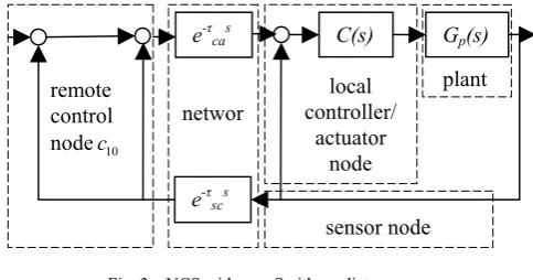
Fig. 3 NCS with new Smith predictor
Gp(s) e-τ
cas C(s)
(a) What time of the remote control node C10 of the event-driven is triggered by the real-time measurement signal from the field sensor, it is completely determined by the delay τsc of the feedback network path. At the same time, the data dropouts in the feedback network path will influence triggered frequency of remote control node C10, further affect control performance of the entire NCS.
(b) What time of the field controller/actuator node of the event-driven is triggered by the remote given reference signal, it is completely determined by the delay τca of the forward network path. Simultaneously, the data dropouts in forward network path will influence triggered frequency of the field controller/actuator node, further affect the control performance of the entire NCS. (c) The remote control node C10 can directly acquire the real-time and on-line measurement signal of the field controlled plant from the field sensor, both can dynamicallyachieve to identify the model parameters of the controlled plant, and can dynamically come true to modify and tune the parameters and states of the field controller/actuator node.
(d) The remote control node C10can take full advantage of the real-time and on-line measurement signal of the field controlled plant from the field sensor, and can implement the complex control algorithms (such as, some advanced control algorithms), simultaneously, can share the real-time and on-line network resources or measurement data with other networked control systems or network nodes together. Even, the output signals of the remote control node C10 can directly be applied to control the field controlled plant. Therefore, its research significance is more important than normal hierarchical control structure. In the hierarchical control structure, the remote control node C10 cannot directly obtain the real-time and on-line measuring signal from the field sensor.
2) The new Smith predictor realizes dynamic prediction compensation for the network delay on structure. The delay of the forward network path is removed from the closed loop, and appears as gain block before the output, and the time-variant uncertain delay in the return network path is totally eliminated from the closed control system. Further, it can cancel the effect of network delays for system stability, and enhances the control performance quality of the entire NCS.
3) Because the delay on the return network path can totally be eliminated, therefore the traffic on the return network path does not need to be scheduled, and the output signal of the field sensor, whenever possible, can directly be transmitted back to remote controller node C10 on the on-line and real-time. On the one hand, this allows utilizing the capacity of the communication channel more effectively than static or dynamic scheduling could. On the other hand, increases system robustness when there are data dropouts on the return network path. 4) The new Smith predictor is the real-time, on-line and
dynamic predictor, and it doesn’t include the prediction models of all network delays on actualization. Because information flow goes through true network delays of the network data transmission process, therefore network delays do not need to be measured, identified or estimated on line. As a consequence, it reduces the
requirement for the node clock synchronization. Furthermore, it avoids estimate errors which are brought due to inaccurate delay model, and avoids node memory resources to be wasted when the network delays are identified or estimated. Simultaneously, it avoids compensation errors, which are brought by the network delays owing to vacancy-sampling and multi-sampling. 5) Because the structure of the new Smith predictor doesn’t include the prediction model of the controlled plant, therefore it doesn’t need to know the exact mathematical model of the controlled plant beforehand. It is particularly applicable to network delay compensation control when the model parameters of the controlled plant are uncertain, unknown or time-variant, or the interference which is inserted to the NCS is difficult to be determined.
6) Because the nodes of the NCS are intelligent nodes [15], it is easy to be realized in the controller, actuator or sensor.
7) The C(s) can adopt PID control, also adopt the intelligent control when the controlled plant is time-variant or nonlinear, and parameter adjustment ofthe C(s) could take no account of the existent of the Smith predictor. D. Nonlinear PID Control
The proportional integral derivative (or PID) control technique has been in existence for over several decades. Up to now, however, this technique is still keeping a dominant role in control engineering, and PID controllers will always remain as a basic element of process control in future, even the other advanced control techniques may appear or mature. Both the past history of control engineering as well as PID control technique itself can support this belief. PID control takes the advantages of the “feedback” idea with most intuitive yet simplest means. As long as the feedback control remains, the principle of PID will be behind in working either explicitly or implicitly, or at least partially.
Because of the changes of the network load or bandwidth, or owing effect of the interference, the parameters of controlled plant could be changed, and control process has different dynamic characteristics, therefore the PID controller parameters should be tuned dynamically. In order to adapt the variation of the network circumstance, a nonlinear PID controller is designed. It comes true to tune the parameters of PID controller automatically. With this strategy, the performance of the NCS is improved.
In the nonlinear PID controller, when the error between the commanded and actual values of the controlled variable is large, the gain amplifies the error substantially to generate a large corrective action to drive the system output to its goal rapidly. As the error diminishes, the gain is automatically reduced to prevent large overshoots in the response. Because of this automatic gain adjustment, the nonlinear PID controller enjoys the advantage of high initial gain to obtain a fast response, followed by a low gain to prevent large overshoots. Its gain adjustment is given as follows [16] 1) Proportional gain kp(ep)
The deviation function of the proportional gain kp(ep) is defined by
(
)
( ( )) 1 sec ( ( ))
p p p p p p
k e t =a +b − h c e t
Where ap, bpand cp are user-defined positive constants, and ep is the error. When error ep → ±∞, the gain kp(ep) takes the maximum (ap + bp). when error ep=0, the gain kp(ep) takes the minimum ap. The bp expresses to change range of the kp(ep). The size of the cp is changed in order to adjust the rate changed of the kp(ep).
2) Integral gain kd(ep)
The function of the integral gain ki(ep) is defined by
( ( )) sec ( ( ))
i p i i p
k e t =a h c e t (7)
Where ai is user-defined positive constants, and the changing range of the ki(ep) is from 0 to ai. When error ep =0, the ki(ep) takes the minimum. The size of the ci is changed in order to adjust the rate changed of the ki(ep).
3) Derivative gain kd(ep)
The function of the derivative gain kd(ep) is defined by
( ( )) / (1 ( ( )))
d p d d d d p
k e t =a +b +c exp d e t⋅ ⋅ (8)
Where ad and bd, cd and dd are user-defined the positive constants, the ad is minimum of the kd(ep), and the maximum of the kd(ep)is sum of the ap and bd .When error ep =0, kd(ep)= ad + bd/(1+ cd). The size of the dd is changed in order to adjust the rate changed of the kd(ep).
The controller algorithm of the nonlinear PID is given by
(
)
(
)
(
)
0
( )
( ) ( ) ( ) ( ) ( ) ( )
t
p
p p p i p p d p
de t u t k e t e t k e t e t dt k e t
dt
= +
∫
+(9) In the real control process, the deviation ep of the given and practical signal values is changing along with operating condition. In the above-mentioned system, the parameters of kp(ep), ki(ep) and kd(ep) are always adjusted to follow deviation automatically. In other words, this nonlinear PID controller is a controller that can change control structure and adaptively tune parameter of the controller. Therefore, this algorithm strengthens the control system robustness.
III. SIMULATION EXPERIMENT
A. Simulation Design
We select the simulation software TrueTime1.5 [17], and the network is CSMA/AMP (CAN bus). The NCS is composed by the network, sensor, controller, actuator, interference nodes and the controlled plants. The data rate is 80,000 bits/s, and minimum frame size is 40 bits in the network. There are some data dropouts in the closed loop, and loss probability is 0.15. The sampling period of the sensor is 0.01 s. The reference signal r adopts square wave and its amplitude is from −1 to 1.
We selected two selfsame controlled plant1 and plant2, and they are second-order plus dead time delay systems as follows
0.01 2
180 ( )
25 1
ps s
p
G s e e
s s
τ
− = −
+ + (10) The plant1 is controlled by the nonlinear PID controller, and
its output is the y1. The plant2 is controlled by the new Smith predictor plus nonlinear PID controller, and its output is y2. In order to research system robustness, we selected controlled plant3 as follows
3 0.02
3 2
200 ( )
20 4
ps s
p
G s e e
s s
τ
− = −
+ + (11) The plant3 is controlled by the new Smith predictor plus nonlinear PID controller, and its output is the y3.
However, all tuned parameters of nonlinear PID controllers completely depend on the (10), where nonlinear PID controllerparameters: ap = 0.95, bp =0.01, cp = 0.8; ai = 0.15, ci = 1.8; ad = 0. 15, bd = 0.135, cd = 3.2, dd= 0.055.
In the simulation process, the data of the sampling and control are encapsulated in the same data package for network transmission, and a step disturbance signal, which amplitude is 0.3, is inserted in output sides of controlled plants at 9.2s.
B. Result Analysis
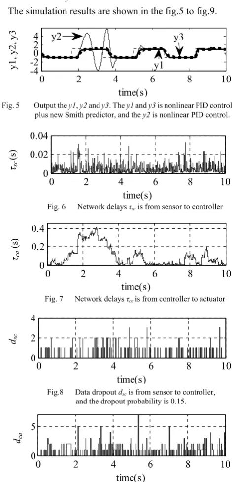
The simulation results are shown in the fig.5 to fig.9.
0 2 4 6 8 10
-4 -20 2 4
time(s)
y2 y3
y1
0 2 4 6 8 10
0 0.02 0.04
time(s)
0 2 4 6 8 10
0 0.2 0.4
time(s)
0 2 4 6 8 10
0 2 4
time(s)
0 2 4 6 8 10
0 5
time(s)
Fig.8 Data dropout dsc is from sensor to controller, and the dropout probability is 0.15.
[image:4.595.307.543.293.782.2]Fig. 6 Network delays τsc is from sensor to controller Fig. 5 Output the y1, y2 and y3. The y1 and y3 is nonlinear PID control
plus new Smith predictor, and the y2 is nonlinear PID control.
Fig. 7 Network delays τca is from controller to actuator
y1, y2, y3
τsc
(s)
τca
(s)
dsc
From the fig.5 to fig.9, we can see
1) The τsc and τca are time variant and uncertain. The maximum of the τsc is 0.033s, it exceeds 3 sampling periods (one sampling period is 0.010s).
2) The data dropout dsc maximum is 4, and the dca is 7. Their dropout probability is 0.15, and lost messages consume the network bandwidth, but never arrive at the destination.
3) The y1 (thick real line) and y3 (thick dot line) are timely in tracking square wave in the fig.5, and their overshoots are less. Therefore, they completely satisfy performance requirements of the NCS. Simultaneously, it also indicates that systems with new Smith predictor have stronger robustness although the model parameters of the plant1 and plant3 have difference.
4) The y2 (in the fig.5, filament) gives after 2.180s, along with increasing and fluctuating of the network delay and data dropout, its overshoot gradually increases from 2.180s to 4.090s, and its control quality is poor. Therefore, the y2 doesn’t satisfy performance requirements of the NCS.
5) After a step disturbance signal, which amplitude is 0.3, is inserted in output sides of the controlled plants at 9.20s. The y1, y2 and y3 can quickly reinstate and track up reference signal. Therefore, it indicates that systems with nonlinear control have stronger anti-jamming ability.
Simulation results show that new Smith predictor combined with nonlinear PID control is effective.
IV. CONCLUSION
In order to effectively restrain the impact of network delay, a novel approach is proposed that new Smith predictor combined with nonlinear control for the NCS. It comes true compensation network delays on structure. This new Smith predictor hides predictor models of the network delays into real network data transmission processes, further the network delays no longer need to be measured, identified or estimated on-line. The structure of new Smith predictor is simple, and has stronger robustness, therefore it is easy to be implemented, and will have wide engineering application prospect.
REFERENCES
[1] H.C. Yan and Max Q. H. Meng, X.H. Huang, “Modeling and robust stability criterion of uncertain networked control systems with time-varying delays”, Proceedings of the 7th World Congress on Intelligent Control and Automation, June 25-27, 2008, Chongqing. China. pp. 188–192.
[2] J. R. Moyne, D. M. Tilbury, “The emergence of industrial control networks for manufacturing control, diagnostics, and safety data”, Vol. 95, No. 1, January 2007 /Proceedings of the IEEE, pp. 29–47. [3] Y. Ge, Q.G. Chen and M. Jiang, Z.A. Liu, “Stability of networked
control systems based on hidden Markova models,” Proceedings of the 7th World Congress on Intelligent Control and Automation June
25-27, 2008, Chongqing, China. pp. 5453–5456.
[4] J. Nilsson, “Real-time control systems with delays,” Ph.D. dissertation, Department of Automatic Control, Lund Institute of Technology, Lund, Sweden, January 1998.
[5] W. Zhang, “Stability analysis of networked control systems,” PhD Thesis, Case Western Reserve University, 2001.
[6] M. Mukai, and M. Fujita, “On networked LQG control with varying delay using the data operator,” Proceedings of the 44th SICE Annual Conference (SICE2005), Okayama, Japan, pp. 3443–3448, 2005.
[7] M. Yu, L. Wang, and T. Chu, “An LMI approach to robust stabilization of networked control systems,” Proceedings of the 16th IFAC World Congress, pp. 3545–3550, July 2005.
[8] Q. Zhu, G. Lu, J. Cao, and S. Hu, “Stability analysis of networked control systems with Markova delay,” Proceedings of 2005
International Conference on Control and Automation (ICCA2005),
Budapest, Hungary, pp. 720–724, June 2005.
[9] L. Liu, C. Tong, and H. Zhang, “Analysis and design of networked control systems with long delays based on Markovian jump model,” Proceedings of the 4th International Conference on Machine Learning and Cybernetics, Guangzhou, China, pp. 953–959, August 2005.
[10] J. Wu, and F. Deng, “Finite horizon optimal control of networked control systems with Markov delays,” Proceedings of the 6th World Congress on Intelligent Control and Automation, Dalian, China, vol. 6, 2006, pp. 4513–4517, June 2006.
[11] Y. L. Wang and G. H. Yang, “H∞ control of networked control systems with time delay and packet disordering, ” IET Control Theory Applications, vol. 1, no. 5, 2007, pp. 1344–1354.
[12] G. P. Liu, Y. Q. Xia, D. Rees and W. S. Hu, “Design and stability criteria of networked predictive control systems with random network delay in the feedback channel, ” IEEE Transactions on Systems, Man, and Cybernetics-Part C: Applications and Reviews, vol. 37, no. 2, 2007, pp. 173–184.
[13] S. Johannessen. “Time synchronization in a local area network,” IEEE Control Syst. Mag., 24: 61–69, 2004
[14] M. Y. Chow, Y. Tipsuwan, “Network-based control systems: A tutorial,” In Proceedings of IECON'OI: The 27th Annual Conference of the IEEE Industrial Electronics Society, pp. 1593–1602, 2001. [15] M.Cakmakci, A.G.Ulsoy, “Bi-directional communication among
“smart” components in a networked control system,” 2005 American
Control Conference, June 8-10. Portland, OR, USA. pp. 627–632,
2005.
[16] J. K. Liu, “Advanced PID control and MATLAB simulation (second edition),” Publish House Electronic industry, Beijing, 2005. [17] O. L. Martin, H.K. Dan, C. Anton. “TrueTime 1.5-reference manual,”
Department of Automatic Control, Lund University, Sweden, January, 2007.