Revealing the Structure of Medical Dictations with Conditional Random Fields

Revealing the Structure of Medical Dictations

with Conditional Random Fields

Jeremy Jancsary and Johannes Matiasek

Austrian Research Institute for Artificial Intelligence A-1010 Vienna, Freyung 6/6

[email protected]

Harald Trost

Department of Medical Cybernetics and Artificial Intelligence of the Center for Brain Research, Medical University Vienna, Austria

[email protected]

Abstract

Automatic processing of medical dictations poses a significant challenge. We approach the problem by introducing a statistical frame-work capable of identifying types and bound-aries of sections, lists and other structures occurring in a dictation, thereby gaining ex-plicit knowledge about the function of such elements. Training data is created semi-automatically by aligning a parallel corpus of corrected medical reports and correspond-ing transcripts generated via automatic speech recognition. We highlight the properties of our statistical framework, which is based on conditional random fields (CRFs) and im-plemented as an efficient, publicly available toolkit. Finally, we show that our approach is effective both under ideal conditions and for real-life dictation involving speech recog-nition errors and speech-related phenomena such as hesitation and repetitions.

1 Introduction

It is quite common to dictate reports and leave the typing to typists – especially for the medical domain, where every consultation or treatment has to be doc-umented. Automatic Speech Recognition (ASR) can support professional typists in their work by provid-ing a transcript of what has been dictated. However, manual corrections are still needed. In particular, speech recognition errors have to be corrected. Fur-thermore, speaker errors, such as hesitations or rep-etitions, and instructions to the transcriptionist have to be removed. Finally, and most notably, proper structuring and formatting of the report has to be

performed. For the medical domain, fairly clear guidelines exist with regard to what has to be dic-tated, and how it should be arranged. Thus, missing headings may have to be inserted, sentences must be grouped into paragraphs in a meaningful way, enu-meration lists may have to be introduced, and so on. The goal of the work presented here was to ease the job of the typist by formatting the dictation ac-cording to its structure and the formatting guide-lines. The prerequisite for this task is the identifi-cation of the various structural elements in the dic-tation which will be be described in this paper.

complaint dehydration weakness and diarrhea full stop Mr. Will Shawn is a 81-year-old cold Asian gentleman who came in with fever and Persian diaper was sent to the emergency department by his primary care physician due him being dehydrated period . . . neck physical exam general alert and oriented times three known acute distress vital signs are stable . . . diagnosis is one chronic diarrhea with hydration he also has hypokalemia neck number thromboctopenia probably duty liver cirrhosis . . . a plan was discussed with patient in detail will transfer him to a nurse and facility for further care . . . end of dictation

Fig. 1: Raw output of speech recognition

Figure 1 shows a fragment of a typical report as recognized by ASR, exemplifying some of the prob-lems we have to deal with:

• Punctuation and enumeration markers may be dictated or not, thus sentence boundaries and numbered items often have to be inferred;

• the same holds for (sub)section headings;

• finally, recognition errors complicate the task.

CHIEF COMPLAINT

Dehydration, weakness and diarrhea.

HISTORY OF PRESENT ILLNESS

Mr. Wilson is a 81-year-old Caucasian gentleman who came in here with fever and persistent diarrhea. He was sent to the emergency department by his primary care physician due to him being dehydrated. . . .

PHYSICAL EXAMINATION

GENERAL: He is alert and oriented times three, not in acute distress.

VITAL SIGNS: Stable. . . .

DIAGNOSIS

1. Chronic diarrhea with dehydration. He also has hypokalemia.

2. Thromboctopenia, probably due to liver cirrhosis.

. . .

PLAN AND DISCUSSION

The plan was discussed with the patient in detail. Will transfer him to a nursing facility for further care.

. . .

Fig. 2: A typical medical report

When properly edited and formatted, the same dictation appears significantly more comprehensi-ble, as can be seen in figure 2. In order to arrive at this result it is necessary to identify the inherent structure of the dictation, i.e. the various hierarchi-cally nested segments. We will recast the segmenta-tion problem as a multi-tiered tagging problem and show that indeed a good deal of the structure of med-ical dictations can be revealed.

The main contributions of our paper are as fol-lows: First, we introduce a generic approach that can be integrated seamlessly with existing ASR solu-tions and provides structured output for medical dic-tations. Second, we provide a freely available toolkit for factorial conditional random fields (CRFs) that forms the basis of aforementioned approach and is also applicable to numerous other problems (see sec-tion 6).

2 Related Work

The structure recognition problem dealt with here is closely related to the field of linear text segmen-tation with the goal to partition text into coherent

blocks, but on a single level. Thus, our task general-izes linear text segmentation to multiple levels.

A meanwhile classic approach towards domain-independent linear text segmentation, C99, is pre-sented in Choi (2000). C99 is the baseline which many current algorithms are compared to. Choi’s al-gorithm surpasses previous work by Hearst (1997), who proposed theTexttilingalgorithm. The best re-sults published to date are – to the best of our knowl-edge – those of Lamprier et al. (2008).

The automatic detection of (sub)section topics

plays an important role in our work, since changes of topic indicate a section boundary and appropri-ate headings can be derived from the section type. Topic detection is usually performed using methods similar to those oftext classification(see Sebastiani (2002) for a survey).

Matsuov (2003) presents a dynamic programming algorithm capable of segmenting medical reports into sections and assigning topics to them. Thus, the aims of his work are similar to ours. However, he is not concerned with the more fine-grained elements, and also uses a different machinery.

When dealing with tagging problems, statistical frameworks such as HMMs (Rabiner, 1989) or, re-cently, CRFs (Lafferty et al., 2001) are most com-monly applied. Whereas HMMs are generative models, CRFs are discriminative models that can in-corporate rich features. However, other approaches to text segmentation have also been pursued. E.g., McDonald et al. (2005) present a model based on multilabel classification, allowing for natural han-dling of overlapping or non-contiguous segments.

Finally, the work of Ye and Viola (2004) bears similarities to ours. They apply CRFs to the pars-ing of hierarchical lists and outlines in handwritten notes, and thus have the same goal of finding deep structure using the same probabilistic framework.

3 Problem Representation

For representing our segmentation problem we use a trick that is well-known from chunking and named entity recognition, and recast the problem as a tag-ging problem in the so-calledBIO1 notation. Since we want to assign a type to every segment, OUTSIDE

labels are not needed. However, we perform

seg-1

...

t₁

t₂

t3

t₄

time step

... ... ... ...

...

...

...

...

...

t5

t6

tokens level 1 < level 2 < level 3 < ...

...

B-T3 B-T4

B-T1

I-T3 I-T4

I-T1

I-T3 I-T4

B-T2

I-T3 I-T4

I-T2

B-T3 I-T4

B-T2

I-T3 I-T4

I-T2

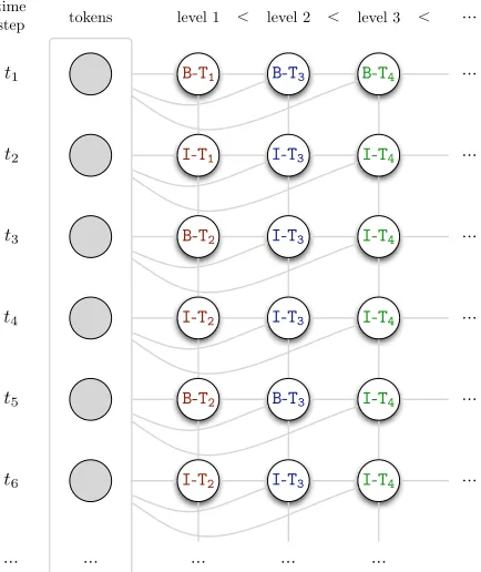
Fig. 3: Multi-level segmentation as tagging problem

mentation on multiple levels, therefore multiple la-bel chainsare required. Furthermore, we also want to assign typesto certain segments, thus the labels need an encoding for the type of segment they rep-resent. Figure 3 illustrates this representation: B-Ti denotes the beginning of a segment of typeTi, while

I-Tiindicates that the segment of typeTicontinues. By adding label chains, it is possible to group the segments of the previous chain into coarser units. Tree-like structures of unlimited depth can be ex-pressed this way2. The gray lines in figure 3 denote dependencies between nodes. Node labels also de-pend on the input token sequence in an arbitrarily wide context window.

4 Data Preparation

The raw data available to us consists of two paral-lel corpora of 2007 reports from the area of medi-cal consultations, dictated by physicians. The first corpus, CRCG, consists of the raw output of ASR

(figure 1), the other one,CCOR, contains the

corre-sponding corrected and formatted reports (figure 2). In order to arrive at an annotated corpus in a

for-2_{Note, that since we omit a redundant top-level chain, this}

structure technically is ahedgerather than atree.

mat suitable for the tagging problem, we first have to analyze the report structure and define appropri-ate labels for each segmentation level. Then, every token has to be annotated with the appropriate begin or inside labels. A report has 625 tokens on average, so the manual annotation of roughly 1.25 million to-kens seemed not to be feasible. Thus we decided to produce the annotations programmatically and re-strict manual work to corrections.

4.1 Analysis of report structure

When inspecting reports inCCOR, a human reader

can easily identify the various elements a report con-sists of, such asheadings– written in bold on a sepa-rate line – introducing sections,subheadings– writ-ten in bold followed by a colon – introducing sub-sections, and enumerations starting with indented numbers followed by a period. Going down further, there areparagraphsdivided intosentences. Using these structuring elements, a hierarchic data struc-ture comprising all report elements can be induced.

Sections and subsections are typed according to their heading. There exist clear recommendations on structuring medical reports, such as E2184-02 (ASTM International, 2002). However, actual med-ical reports still vary greatly with regard to their structure. Using the aforementioned standard, we assigned the (sub)headings that actually appeared in the data to the closest type, introducing new types only when absolutely necessary. Finally we arrived at a structure model with three label chains:

• Sentence level, with 4 labels: Heading,

Subheading,Sentence,Enummarker • Subsection level, with 45 labels: Paragraph,

Enumelement, None and 42 subsection types (e.g.VitalSigns,Cardiovascular...)

• Section level, with 23 section types (e.g.

ReasonForEncounter,Findings,Plan...)

4.2 Corpus annotation

Since the reports inCCOR are manually edited they

CCOR OP CRCG

. . . .

B−Head CHIEF del

Head COMPLAINT sub complaint B−Head B−Sent Dehydration sub dehydration B−Sent

Sent , del

Sent weakness sub weakness Sent

Sent and sub and Sent

Sent diarrhea sub diarrhea Sent

Sent . sub fullstop Sent

B−Sent Mr. sub Mr. B−Sent

Sent Wilson sub Will Sent

ins Shawn Sent

Sent is sub is Sent

Sent a sub a Sent

Sent 81-year-old sub 81-year-old Sent

Sent Caucasian sub cold Sent

Sent ins Asian Sent

Sent gentleman sub gentleman Sent

Sent who sub who Sent

Sent came sub came Sent

Sent in del

Sent here sub here Sent Sent with sub with Sent

Sent fever sub fever Sent

Sent and sub and Sent

Sent persistent sub Persian Sent

Sent diarrhea sub diaper Sent

Sent . del

. . . .

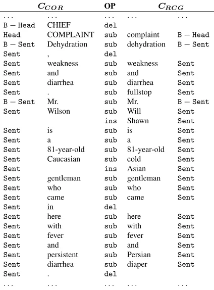
Fig. 4: Mapping labels via alignment

of the parser is a hedge data structure from which the annotation labels can be derived easily.

However, our goal is to develop a model for rec-ognizing the report structure from thedictation, thus we have to map the newly created annotation of re-ports in CCOR onto the corresponding reports in

CRCG. The basic idea here is to align the tokens

ofCCOR with the tokens inCRCG and to copy the

annotations (cf. figure 43). There are some peculiar-ities we have to take care of during alignment:

1. non-dictated items inCCOR (e.g. punctuation,

headings)

2. dictated words that do not occur inCCOR(meta

instructions, repetitions)

3. non-identical but corresponding items (recog-nition errors, reformulations)

Since it is particularly necessary to correctly align items of the third group, standard string-edit dis-tance based methods (Levenshtein, 1966) need to be augmented. Therefore we use a more sophisticated

3_{This approach can easily be generalized to multiple label}

chains.

cost function. It assigns tokens that are similar (ei-ther from a semantic or phonetic point of view) a low cost for substitution, whereas dissimilar tokens re-ceive a prohibitively expensive score. Costs for dele-tion and inserdele-tion are assigned inversely. Seman-tic similarity is computed using Wordnet (Fellbaum, 1998) and UMLS (Lindberg et al., 1993). For pho-netic matching, the Metaphone algorithm (Philips, 1990) was used (for details see Huber et al. (2006)).

4.3 Feature Generation

The annotation discussed above is the first step to-wards building a training corpus for a CRF-based approach. What remains to be done is to provide ob-servations for each time step of the observed entity, i.e. for each token of a report; these are expected to give hints with regard to the annotation labels that are to be assigned to the time step. The observa-tions, associated with one or more annotation labels, are usually calledfeatures in the machine learning literature. During CRF training, the parameters of these features are determined such that they indicate the significance of the observations for a certain la-bel or lala-bel combination; this is the basis for later tagging of unseen reports.

We use the following features for each time step of the reports inCCORandCRCG:

• Lexical featurescovering the local context of

±2tokens (e.g.,patient@0,the@-1,is@1)

• Syntactic featuresindicating the possible syn-tactic categories of the tokens (e.g., NN@0,

JJ@0,DT@-1andbe+VBZ+aux@1)

• Bag-of-word (BOW) features intend to cap-ture the topic of a text segment in a wider context of±10 tokens, without encoding any order. Tokens are lemmatized and replaced by their UMLS concept IDs, if available, and weighed byTF. Thus, different words describ-ing the same concept are considered equal.

• Semantic type features as above, but using UMLS semantic types instead of concept IDs provide a coarser level of description.

5 Structure Recognition with CRFs

Conditional random fields (Lafferty et al., 2001) are conditional models in the exponential family. They can be considered a generalization of multinomial logistic regression to output with non-trivial internal structure, such as sequences, trees or other graphical models. We loosely follow the general notation of Sutton and McCallum (2007) in our presentation.

Assuming an undirected graphical model Gover an observed entity x and a set of discrete, inter-dependent random variables4 y, a conditional ran-dom field describes the conditional distribution:

p(y|x;θ) = 1 Z(x)

Y

c∈G

φ_c(y_c,x;θc) (1)

The normalization termZ(x)sums over all possible joint outcomes ofy, i.e.,

Z(x) =X y0

p(y0|x;θ) (2)

and ensures the probabilistic interpretation of p(y|x). The graphical modelG describes interde-pendencies between the variables y; we can then modelp(y|x)via factorsφ_c(·)that are defined over cliquesc∈G. The factorsφ_c(·)are computed from sufficient statistics{fck(·)}of the distribution

(cor-responding to the features mentioned in the previous section) and depend on possibly overlapping sets of parametersθc ⊆θwhich together form the

param-etersθof the conditional distribution:

φ_c(y_c,x;θc) = exp



 |θc| X

k=1

λckfck(x,yc)



 (3)

In practice, for efficiency reasons, independence as-sumptions have to be made about variablesy ∈ y, so Gis restricted to small cliques (say, (|c| ≤ 3). Thus, the sufficient statistics only depend on a lim-ited number of variablesyc⊆y; they can, however, access the whole observed entityx. This is in con-trast to generative approaches which model a joint distributionp(x,y)and therefore have to extend the independence assumptions to elementsx∈x.

4

In our case, the discrete outcomes of the random variables ycorrespond to the annotation labels described in the previous section.

The factor-specific parameters θc of a CRF are

typically tied for certain cliques, according to the problem structure (i.e., θc1 = θc2 for two cliques

c1, c2 with tied parameters). E.g., parameters are

usually tied across time if G is a sequence. The factors can then be partitioned into a set of clique templatesC ={C1, C2, . . . CP}, where each clique

templateCp is a set of factors with tied parameters

θp and corresponding sufficient statistics{fpk(·)}.

The CRF can thus be rewritten as:

p(y|x) = 1 Z(x)

Y

Cp∈C

Y

φc∈Cp

φ_c(y_c,x;θp) (4)

Furthermore, in practice, the sufficient statistics

{fpk(·)} are computed from a subset xc ⊆ xthat

is relevant to a factorφ_c(·). In a sequence labelling task, tokensx∈xthat are in temporal proximity to an output variabley ∈ y are typically most useful. Nevertheless, in our notation, we will let factors de-pend on the whole observed entityxto denote that all ofxcan be accessed if necessary.

For our structure recognition task, the graphical model G exhibits the structure shown in figure 3, i.e., there are multiple connected chains of variables with factors defined over single-node cliques and two-node cliques within and between chains; the pa-rameters of factors are tied across time. This corre-sponds to the factorial CRF structure described in Sutton and McCallum (2005). Structure recognition using conditional random fields then involves two separate steps:parameter estimation, or training, is concerned with selecting the parameters of a CRF such that they fit the given training data.Prediction, or testing, determines the best label assignment for unknown examples.

5.1 Parameter estimation

Given IID training dataD={x(i),y(i)}N

i=1,

param-eter estimation dparam-etermines:

θ∗ = argmax θ0

N

X

i

p(y(i)|x(i);θ0)

!

(5)

i.e., those parameters that maximize the conditional probability of the CRF given the training data.

In the following, we will not explicitly sum over

N

i=1; as Sutton and McCallum (2007) note, the

We thus assume G and its factors φ_c(·) to extend over all training instances. Unfortunately, (5) cannot be solved analytically. Typically, one performs max-imum likelihood estimation (MLE) by maximizing the conditional log-likelihood numerically:

`(θ) = X

Cp∈C

X

φc∈Cp

|θp| X

k=1

λpkfpk(x,yc)−logZ(x)

(6) Currently, limited-memory gradient-based methods such as LBFGS (Nocedal, 1980) are most com-monly employed for that purpose5. These require the partial derivatives of (6), which are given by:

∂` ∂λpk

= X φc∈Cp

fpk(x,yc)−

X

y0 c

fpk(x,y0c)p(y

0

c|x)

(7) and expose the intuitive form of a difference be-tween the expectation of a sufficient statistic accord-ing to the empiric distribution and the expectation according to the model distribution. The latter term requires marginal probabilities for each cliquec, de-noted byp(y0_c|x). Inference on the graphical model G(see sec 5.2) is needed to compute these.

Depending on the structure ofG, inference can be very expensive. In order to speed up parameter es-timation, which requires inference to be performed for every training example and for every iteration of the gradient-based method, alternatives to MLE have been proposed that do not require inference. We show here a factor-based variant of pseudolike-lihood as proposed by Sanner et al. (2007):

`p(θ) = X

Cp∈C

X

φc∈Cp

logp(y_c|x,MB(φ_c)) (8)

where the factors are conditioned on the Markov blanket, denoted byM B6. The gradient of (8) can be computed similar to (7), except that the marginals pc(y0c|x)are also conditioned on the Markov

blan-ket, i.e.,pc(y0c|x,MB(φc)). Due to its dependence

on the Markov blanket of factors, pseudolikelihood

5

Recently, stochastic gradient descent methods such as On-line LBFGS (Schraudolph et al., 2007) have been shown to per-form competitively.

6

Here, the Markov blanket of a factorφcdenotes the set of variables occurring in factors that share variables withφc, non-inclusive of the variables ofφ_c

cannot be applied to prediction, but only to param-eter estimation, where the “true” assignment of a blanket is known.

5.1.1 Regularization

We employ a Gaussian prior for training of CRFs in order to avoid overfitting. Hence, iff(θ) is the original objective function (e.g., log-likelihood or log-pseudolikelihood), we optimize a penalized ver-sionf0(θ)instead, such that:

f0(θ) =f(θ)−

|θ| X

k=1

λ2_k 2σ2 and

∂f0 ∂λk

= ∂f ∂λk

−λk

σ2.

The tuning parameterσ2 determines the strength of the penalty; lower values lead to less overfitting. Gaussian priors are a common choice for parame-ter estimation of log-linear models (cf. Sutton and McCallum (2007)).

5.2 Inference

Inference on a graphical model G is needed to ef-ficiently compute the normalization termZ(x)and marginalspc(y0c|x)for MLE, cf. equation (6).

Using belief propagation (Yedidia et al., 2003), more precisely its sum-product variant, we can com-pute the beliefs for all cliques c ∈ G. In a tree-shaped graphical modelG, these beliefs correspond exactly to the marginal probabilitiespc(y0c|x).

How-ever, if the graph contains cycles, so-called loopy belief propagation must be performed. The mes-sage updates are then re-iterated according to some schedule until the messages converge. We use a TRP schedule as described by Wainwright et al. (2002). The resulting beliefs are then only approximations to the true marginals. Moreover, loopy belief propa-gation is not guaranteed to terminate in general – we investigate this phenomenon in section 6.5.

5.3 Prediction

Once the parameters θ have been estimated from training data, a CRF can be used to predict the la-bels of unknown examples. The goal is to find:

y∗ = argmax y0

p(y0|x;θ)

(9)

i.e., the assignment ofy that maximizes the condi-tional probability of the CRF. Again, naive computa-tion of (9) is intractable. However, the max-product variant of loopy belief propagation can be applied to approximately find the MAP assignment ofy (max-product can be seen as a generalization of the well-known Viterbi algorithm to graphical models).

For structure recognition in medical reports, we employ a post-processing step after label prediction with the CRF model. As in Jancsary (2008), this step enforces the constraints of theBIOnotation and ap-plies some trivial non-local heuristics that guarantee a consistent global view of the resulting structure.

6 Experiments and Results

For evaluation, we generally performed 3-fold cross-validation for all performance measures. We cre-ated training data from the reports in CCOR so as

to simulate a scenario under ideal conditions, i.e., perfect speech recognition and proper dictation of punctuation and headings, without hesitation or rep-etitions. In contrast, the data from CRCG reflects

real-life conditions, with a wide variety of speech recognition error rates and speakers frequently hes-itating, repeating themselves and omitting punctua-tion and/or headings.

Depending on the experiment, two different sub-sets of the two corpora were considered:

• C{COR,RCG}-ALL: All 2007 reports were used,

resulting in 1338 training examples and 669 testing examples at each CV-iteration.

• C{COR,RCG}-BEST: The corpus was restricted

to those 1002 reports that yielded the lowest word error rate during alignment (see section 4.2). Each CV-iteration hence amounts to 668 training examples and 334 testing examples.

From the crossvalidation runs, a 95%-confidence interval for each measure was estimated as follows:

¯

Y ±t_(α/2,N−1)

s

√

N = ¯Y ±t(0.025,2) s

√

3 (10)

0 10 20 30 40 50 60 70 80 90 100

0 100 200 300 400 500 600 700 800

relative loss / accuracy (%)

number of iterations Loss on training set Accuracy on validation set

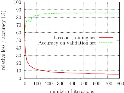
Fig. 5: Accuracy vs. loss function onCRCG-ALL

whereY¯ is the sample mean,sis the sample stan-dard deviation,N is the sample size (3),αis the de-sired significance level (0.05) andt_(α/2,N−1) is the

upper critical value of thet-distribution withN−1 degrees of freedom. The confidence intervals are in-dicated in the±column of tables 1, 2 and 3.

For CRF training, we minimized the penalized, negative log-pseudolikelihood using LBFGS with m = 3. The variance of the Gaussian prior was set toσ2 = 1000. All supported features were used for univariate factors, while the bivariate factors within chains and between chains were restricted to bias weights. For testing, loopy belief propagation with a TRP schedule was used in order to determine the maximum a posteriori (MAP) assignment. We use

VieCRF, our own implementation of factorial CRFs, which is freely available at the author’s homepage7.

6.1 Analysis of training progress

In order to determine the number of required train-ing iterations, an experiment was performed that compares the progress of theAccuracymeasure on a validation set to the progress of the loss function on a training set. The data was randomly split into a training set (2/3 of the instances) and a validation set. Accuracy on the validation set was computed using the intermediate CRF parametersθt every 5

iterations of LBFGS. The resulting plot (figure 5) demonstrates that the progress of the loss function corresponds well to that of theAccuracy measure,

Estimated Accuracies

Acc. ±

Average 97.24% 0.33 Chain 0 99.64% 0.04 Chain 1 95.48% 0.55 Chain 2 96.61% 0.68 Joint 92.51% 0.97

(a)CCOR-ALL

Estimated Accuracies

Acc. ±

Average 86.36% 0.80 Chain 0 91.74% 0.16 Chain 1 85.90% 1.25 Chain 2 81.45% 2.14 Joint 69.19% 1.93

(b)CRCG-ALL

Table 1: Accuracy on the full corpus

Estimated Accuracies

Acc. ±

Average 96.48% 0.82 Chain 0 99.55% 0.08 Chain 1 94.64% 0.23 Chain 2 95.25% 2.16 Joint 90.65% 2.15

(a)CCOR-BEST

Estimated Accuracies

Acc. ±

Average 87.73% 2.07 Chain 0 93.77% 0.68 Chain 1 87.59% 1.79 Chain 2 81.81% 3.79 Joint 70.91% 4.50

(b)CRCG-BEST

Table 2: Accuracy on a high-quality subset

thus an “early stopping” approach might be tempt-ing to cut down on traintempt-ing times. However, durtempt-ing earlier stages of training, the CRF parameters seem to be strongly biased towards high-frequency labels, so other measures such as macro-averagedF1might suffer from early stopping. Hence, we decided to allow up to 800 iterations of LBFGS.

6.2 Accuracy of structure prediction

Table 1 shows estimated accuracies forCCOR-ALL

and CRCG-ALL. Overall, high accuracy (> 97%)

can be achieved onCCOR-ALL, showing that the

ap-proach works very well under ideal conditions. Per-formance is still fair on the noisy data (CRCG-ALL;

Accuracy > 86%). It should be noted that the la-bels are unequally distributed, especially inchain 0

(there are very few BEGINlabels). Thus, the

base-line is substantially high for this chain, and other measures may be better suited for evaluating seg-mentation quality (cf. section 6.4).

6.3 On the effect of noisy training data

Measuring the effect of the imprecise reference an-notation ofCRCG is difficult without a

correspond-ing, manually created golden standard. However, to get a feeling for the impact of the noise induced by speech recognition errors and sloppy dictation

Estimated WD

WD ±

Chain 0 0.007 0.000 Chain 1 0.050 0.007 Chain 2 0.015 0.001

(a)CCOR-ALL

Estimated WD

WD ±

Chain 0 0.193 0.008 Chain 1 0.149 0.005 Chain 2 0.118 0.013

(b)CRCG-ALL

Table 3: Per-chainWindowDiffon the full corpus

on the quality of the semi-automatically generated annotation, we conducted an experiment with sub-setsCCOR-BEST andCRCG-BEST. The results are

shown in table 2. Comparing these results to ta-ble 1, one can see that overall accuracydecreased

for CCOR-BEST, whereas we see an increase for

CRCG-BEST. This effect can be attributed to two

different phenomena:

• InCCOR-BEST, no quality gains in the

anno-tation could be expected. The smaller number of training examples therefore results in lower accuracy.

• Fewer speech recognition errors and more con-sistent dictation inCRCG-BEST allow for

bet-ter alignment and thus a betbet-ter reference anno-tation. This increases the actual prediction per-formance and, furthermore, reduces the num-ber of label predictions that are erroneously counted as a misprediction.

Thus, it is to be expected that manual correction of the automatically created annotation results in sig-nificant performance gains. Preliminary annotation experiments have shown that this is indeed the case.

6.4 Segmentation quality

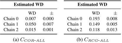
Accuracyis not the best measure to assess segmen-tation quality, therefore we also conducted experi-ments using theWindowDiff measure as proposed by Pevzner and Hearst (2002). WindowDiff re-turns 0 in case of a perfect segmentation; 1 is the worst possible score. However, it only takes into account segment boundaries and disregards segment types. Table 3 shows the WindowDiff scores for CCOR-ALL andCRCG-ALL. Overall, the scores are

quite good and are consistently below0.2. Further-more,CRCG-ALLscores do not suffer as badly from

Converged (%) Iterations (∅)

CCOR-ALL 0.999 15.4

CRCG-ALL 0.911 66.5

CCOR-BEST 0.999 14.2

CRCG-BEST 0.971 37.5

Table 4: Convergence behaviour of loopy BP

6.5 Convergence of loopy belief propagation

In section 5.2, we mentioned that loopy BP is not guaranteed to converge in a finite number of itera-tions. Since we optimize pseudolikelihood for pa-rameter estimation, we are not affected by this limi-tation in the training phase. However, we use loopy BP with a TRP schedule during testing, so we must expect to encounter non-convergence for some ex-amples. Theoretical results on this topic are dis-cussed by Heskes (2004). We give here an empir-ical observation of convergence behaviour of loopy BP in our setting; the maximum number of itera-tions of the TRP schedule was restricted to 1,000. Table 4 shows the percentage of examples converg-ing within this limit and the average number of iter-ations required by the converging examples, broken down by the different corpora. From these results, we conclude that there is a connection between the quality of the annotation and the convergence be-haviour of loopy BP. In practice, even though loopy BP didn’t converge for some examples, the solutions after 1,000 iterations where satisfactory.

7 Conclusion and Outlook

We have presented a framework which allows for identification of structure in report dictations, such as sentence boundaries, paragraphs, enumerations, (sub)sections, and various other structural elements; even if no explicit clues are dictated. Furthermore, meaningful types are automatically assigned to sub-sections and sub-sections, allowing – for instance – to automatically assign headings, if none were dic-tated.

For the preparation of training data a mechanism has been presented that exploits the potential of par-allel corpora for automatic annotation of data. Us-ing manually edited formatted reports and the cor-responding raw output of ASR, reference annotation can be generated that is suitable for learning to

iden-tify structure in ASR output.

For the structure recognition task, a CRF frame-work has been employed and multiple experiments have been performed, confirming the practicability of the approach presented here.

One result deserving further investigation is the effect of noisy annotation. We have shown that segmentation results improve when fewer errors are present in the automatically generated annotation. Thus, manual correction of the reference annotation will yield further improvements.

Finally, the framework presented in this paper opens up exciting possibilities for future work. In particular, we aim at automatically transform-ing report dictations into properly formatted and rephrased reports that conform to the requirements of the relevant domain. Such tasks are greatly facili-tated by the explicit knowledge gained during struc-ture recognition.

Acknowledgments

The work presented here has been carried out in the context of the Austrian KNet competence net-work COAST. We gratefully acknowledge funding by the Austrian Federal Ministry of Economics and Labour, and ZIT Zentrum fuer Innovation und Tech-nologie, Vienna. The Austrian Research Institute for Artificial Intelligence is supported by the Aus-trian Federal Ministry for Transport, Innovation, and Technology and by the Austrian Federal Ministry for Science and Research.

Furthermore, we would like to thank our anony-mous reviewers for many insightful comments that helped us improve this paper.

References

ASTM International. 2002. ASTM E2184-02: Standard specification for healthcare document formats. Freddy Choi. 2000. Advances in domain independent

linear text segmentation. In Proceedings of the first conference on North American chapter of the Associa-tion for ComputaAssocia-tion Linguistics, pages 26–33. C. Fellbaum. 1998. WordNet: an electronic lexical

database. MIT Press, Cambridge, MA.

Tom Heskes. 2004. On the uniqueness of loopy belief propagation fixed points. Neural Comput., 16(11):2379–2413.

Martin Huber, Jeremy Jancsary, Alexandra Klein, Jo-hannes Matiasek, and Harald Trost. 2006. Mismatch interpretation by semantics-driven alignment. In Pro-ceedings of KONVENS ’06.

Jeremy M. Jancsary. 2008. Recognizing structure in re-port transcripts. Master’s thesis, Vienna University of Technology.

John Lafferty, Andrew McCallum, and Fernando Pereira. 2001. Conditional Random Fields: Probabilistic mod-els for segmenting and labeling sequence data. In Pro-ceedings of the Eighteenth International Conference on Machine Learning (ICML).

S. Lamprier, T. Amghar, B. Levrat, and F. Saubion. 2008. Toward a more global and coherent segmen-tation of texts. Applied Artificial Intelligence, 23:208– 234, March.

Vladimir I. Levenshtein. 1966. Binary codes capable of correcting deletions, insertions and reversals. Soviet Physics Doklady, 10(8):707–710.

D. A. B. Lindberg, B. L. Humphreys, and A. T. McCray. 1993. The Unified Medical Language System. Meth-ods of Information in Medicine, 32:281–291.

Evgeny Matsuov. 2003. Statistical methods for text segmentation and topic detection. Master’s the-sis, Rheinisch-Westf¨alische Technische Hochschule Aachen.

Ryan McDonald, Koby Crammer, and Fernando Pereira. 2005. Flexible text segmentation with structured multilabel classification. In Proceedings of Human Language Technology Conference and Conference on Empirical Methods in Natural Language Processing (HLT/EMNLP), pages 987–994.

Jorge Nocedal. 1980. Updating Quasi-Newton matri-ces with limited storage. Mathematics of Computa-tion, 35:773–782.

Lev Pevzner and Marti Hearst. 2002. A critique and improvement of an evaluation metric for text segmen-tation. Computational Linguistics, 28(1), March. Lawrence Philips. 1990. Hanging on the metaphone.

Computer Language, 7(12).

L. R. Rabiner. 1989. A tutorial on hidden Markov mod-els and selected applications in speech recognition. Proceedings of the IEEE, 77:257–286, February. Scott Sanner, Thore Graepel, Ralf Herbrich, and Tom

Minka. 2007. Learning CRFs with hierarchical fea-tures: An application to go. International Conference on Machine Learning (ICML) workshop.

Nicol N. Schraudolph, Jin Yu, and Simon G¨unter. 2007. A stochastic Quasi-Newton Method for online convex optimization. In Proceedings of 11th International Conference on Artificial Intelligence and Statistics.

Fabrizio Sebastiani. 2002. Machine learning in auto-mated text categorization. ACM Computing Surveys, 34(1):1–47.

Charles Sutton and Andrew McCallum. 2005. Composi-tion of CondiComposi-tional Random Fields for transfer learn-ing. InProceedings of Human Language Technologies / Empirical Methods in Natural Language Processing (HLT/EMNLP).

Charles Sutton and Andrew McCallum. 2007. An intro-duction to Conditional Random Fields for relational learning. In Lise Getoor and Ben Taskar, editors, Introduction to Statistical Relational Learning. MIT Press.

Martin Wainwright, Tommi Jaakkola, and Alan S. Will-sky. 2002. Tree-based reparameterization framework for analysis of sum-product and related algorithms. IEEE Transactions on Information Theory, 49(5). Ming Ye and Paul Viola. 2004. Learning to parse

hi-erarchical lists and outlines using Conditional Ran-dom Fields. InProceedings of the Ninth International Workshop on Frontiers in Handwriting Recognition (IWFHR’04), pages 154–159. IEEE Computer Soci-ety.