Sentence ordering with manifold based classification in multi document summarization

Sentence Ordering with Manifold-based Classification in

Multi-Document Summarization

Paul D Ji

Centre for Linguistics and Philology University of Oxford

[email protected]

Stephen Pulman

Centre for Linguistics and Philology University of Oxford

[email protected]

Abstract

In this paper, we propose a sentence ordering algorithm using a semi-supervised sentence classification and historical ordering strategy. The classification is based on the manifold structure underlying sentences, addressing the problem of limited labeled data. The historical ordering helps to ensure topic continuity and avoid topic bias. Experiments demonstrate that the method is effective.

1. Introduction

Sentence ordering has been a concern in text planning and concept-to-text generation (Reiter et al., 2000). Recently, it has also drawn attention in multi-document summarization (Barzilay et al., 2002; Lapata, 2003; Bollegala et al., 2005). Since summary sentences generally come from different sources in multi-document summarization, an optimal ordering is crucial to make summaries coherent and readable.

In general, the strategies for sentence ordering in multi-document summarization fall in two categories. One is chronological ordering (Barzilay et al., 2002; Bollegala et al., 2005), which is based on time-related features of the documents. However, such temporal features may be not available in all cases. Furthermore, temporal inference in texts is still a problem, in spite of some progress in automatic disambiguation of temporal information (Filatova

et al., 2001).

Another strategy is majority ordering (MO) (McKeown et al., 2001; Barzilay et al., 2002), in which each summary sentence is mapped to a theme, i.e., a set of similar sentences in the documents, and the order of these sentences determines that for summary sentences. To do that, a directed theme graph is built, in which if a theme A occurs behind another theme B in a document, B is linked to A no matter how far away they are located. However, this may lead to wrong theme correlations, since B’s occurrence may rely on a third theme C and have nothing to do with A. In addition, when outputting theme orders, MO uses a kind of heuristic that chooses a theme based on its in-out edge difference in the directed theme graph. This may cause topic disruption, since the next choice may have no link with previous choices.

strategy helps to ensure continuity of topics but to avoid topic bias at the same time.

To do that, we need to map summary sentences to those in documents. We formalize this as a kind of classification problem, with summary sentences as class labels. Since there are very few (only one) labeled examples for each class, we adopt a kind of semi-supervised classification method, which makes use of the manifold structure underlying the sentences to do the classification. A common assumption behind this learning paradigm is that the manifold structure among the data, revealed by higher density, provides a global comparison between data points (Szummer et al., 2001; Zhu et al., 2003; Zhou et al., 2003). Under such an assumption, even one labeled example is enough for classification, if only the structure is determined.

The remainder of the paper is organized as follows. In section 2, we give an overview of the proposed method. In section 3~5, we talk about the method including sentence networks, classification and ordering. In section 6, we present experiments and evaluations. Finally in section 7, we give some conclusions and future work.

2. Overview

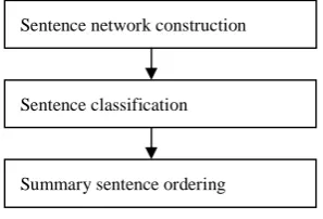
Fig. 1 gives the overall structure of the proposed method, which includes three modules: construction of sentence networks, sentence classification and sentence ordering.

Fig. 1. Algorithm Overview

The first step is to build a sentence neighborhood

network with weights on edges, which can serve as the basis for a Markov random walk (Tishby et al., 2000). The neighborhood is based on similarity between sentences, and weights on edges can be seen as transition probabilities for the random walk. From this network, we can derive new representations for sentences. The second step is to make a classification of sentences, with each summary sentence as a class label. Since only one labeled example exists for each class, we use a semi-supervised method based on a Markov random walk to reveal the manifold structure for the classification.

The third step is to order summary sentences according to the original positions of their partners in the same class. During this process, the next selection of a sentence is based on the whole history of selection, i.e., the association of the sentence with all those already selected.

3. Sentence Network Construction

Suppose S is the set of all sentences in the documents and a summary (a summary sentence may be not a document sentence), let S={s1,

s2, …, sN} with a distance metric d(si,sj), the distance between two sentences si and sj, which is based on the Jensen-Shannon divergence (Lin, 1991). We construct a graph with sentences as points by sorting the distances among the points in an ascending order and repeatedly connecting two points according to the order until a connected graph is obtained. Then, we assign a weight wi,j, as in (1), to each edge based on the distance.

) / ) , ( exp( )

1 wi,j = −d si sj

δ

The weights are symmetric, wi,i=1 and wi,j=0 for all non-neighbors (δ is set as 0.6 in this work). 2) is the one-step transition probability p(si, sj) from

si to sj based on weights of neighbors.

∑

=

k k i j i j

i

w w s

s p

, ,

) , ( ) 2 Sentence network construction

Sentence classification

Let M be the N×N matrix and Mi,j= p(si, sj), then Mt is the tth Markov random walk matrix, whose i,

j-th entry is the probability pt(si, sj) of the transition from si to sj after t steps. In this way, each sentence sj is associated with a vector of conditional probabilities pt(si, sj), i=1, …, N, which form a new manifold-based representation for sj. With such representations, sentences are close whenever they have a similar distribution over the starting points. Notice that the representations depend on the step parameter t (Tishby et al., 2000). With smaller values of t, unlabeled points may be not connected with labeled ones; with bigger values of t, the points may be indistinguishable. So, an appropriate t should be estimated.

4. Sentence Classification

Suppose s1, s2, …, sL are summary sentences and their labels are c1, c2, …, cL respectively. In our case, each summary sentence is assigned with a unique class label ci, 1≤i≤L. This also means that for each class ci, there is only one labeled example, i.e., the summary sentence, si.

Let S={(s1, c1), (s2, c2), …, (sL, cL), sL+1,…, sN}, then the task of sentence classification is to infer the labels for unlabeled sentences, sL+1,…, sN. Through the classification, we can get similar sentences for each summary sentence. To do that, we assume that each sentence has a distribution

p(ck|si), 1≤k≤L, 1≤i≤N, and these probabilities are to be estimated from the data.

Seeing a sentence as a sample from the t step Markov random walk in the sentence graph, we have the following interpretation of p(ck|si).

∑

k s p c s p j i

c

p( | ) ( | ) ( , )

) 3

This means that the probability of si belonging to ck is dependent on the probabilities of those sentences belonging to ck which will transit to si after t steps and their transition probabilities. With the conditional log-likelihood of labeled sentences 4) as the estimation criterion, we can

use the EM algorithm to estimate p(ck|si), in which the E-step and M-step are 5) and 6) respectively.

∑

∑

∑

k s p c s p j k

c p

1 1 1

) , ( ) | ( log ) | ( log ) 4

∑

i s c pc s p i k pc s p i k s p 1 ) , ( ) | ( / ) , ( ) | ( ) , | ( ) 5

∑

k s p s s c p s s c

c p 1 ) , | ( / ) , | ( ) | ( ) 6

The final class ci for si is given in 7).

) | ( max arg )

7 c_{i c} p c_k s_i

k

=

p(ci|si) is called the membership probability of si. After classification, each sentence is assigned a label according to 7).

One key problem in this setting is to estimate the parameter t. A possible strategy for that is by cross validation, but it needs a large amount of labeled data. Here, following Szummer et al., 2001, we use marginal difference of probabilities of sentences falling in different classes as the estimation criterion, which is given in 8).

∑

∑

∈ ≤ ≤ ≤ ≤

− =

S

s k L

k k

L

k p c s p c s

L S

m

1

1 ( | ) ( | ))

max ( ) ( ) 8

To maximize 8), we can get an appropriate value for the parameter t, which means that a better t should make sentences belong to some classes more prominently. Notice that the classes represented by summary sentences may be incomplete for all the sentences occurring in the documents, so some sentences will belong to the classes without obviously different probabilities. To avoid such sentences in the estimation of t, we only choose the top (40%) sentences in a class based on their membership probabilities.

5. Sentence Ordering

node, and there exists a directed edge ei,j from one node ci to another cj if and only if there is si in ci immediately appearing before sj in cj in the documents (the sentences not in classes are neglected). The weight of ei,j, Fi,j, captures the frequency of such occurrence. We add one additional node denoting an initial class c0, and it links to each class with a directed edge e0,j, the weight F0,j of which is the frequency of the member sentences of the class appearing at the beginning of the documents.

Suppose the input is the class graph G=<C, E>, where C = {c1, c2, …, cL} is the set of the classes,

E={ei,j|1≤i, j≤L} is the set of the directed edges, and o is the ordering of the classes. Fig. 2 gives the ordering algorithm.

---

i) _i

C c

k F

c

i , 0

max

∈

←

ii) o← o ck

iii) For all ci in C,F_0,i ←F_0,i +F_k,i iv) Remove ck from C and ek,j and ei,k from E; v) Repeat i)-iv) while C≠{ c0}

vi) Return the order o.

---

Fig. 2 Ordering algorithm

In the algorithm, there are two main steps. Step i) selects the class whose member sentences occur most frequently immediately after those in c0. Step iii) updates the weights of the edges e0,i. In fact, it can be seen as merge of the original c0 and

ck, and in this sense the updated c0 represents the history of selections.

In contrast to the MO algorithm, the ordering algorithm here (HO) uses immediate back-front co-occurrence, while the MO algorithm uses relative back-front locations. On the other hand, the selection of a class is dependent on previous selections in HO, while in MO, the selection of a class is mainly dependent on its in-out edge difference.

In contrast to the PO algorithm, the selection of a class in HO is dependent on all previous selections, while in PO, the selection is only

related to the most recent one.

As an example, Fig. 3 gives an initial class graph. The output orderings by PO and HO are [c1, c3, c4, c2] and [c1, c3, c2, c4] respectively. The difference lies in whether to select c4 or c2 after selection of c3. PO selects c4 since it only considers the most recent selection, while HO selects c2 because it considers all previous selections including c1.

c0

9

c1

5 6

c2 c3

1 2

1 c4

Fig. 3 Initial graph for PO and HO

As another example, Fig. 4 gives the order of the classes in individual documents.

1) c2 c3 c1

2) c2 c3 c1

3) c3 c2 c1

4) c3 c2 c1

5) c3 c2

6) c2 c3

7) c1 c2 c3 c2 c3 c2 c3 c2

Fig. 4. Class orders in documents

From 1)-6), we can see some regularity among the order of the classes: c2 and c3 are interchangeable, while c1 always appears behind

c2 or c3. From 7), we can see that c2 and c3 still co-occur, while c1 happens to occur at the beginning of the document. Thus, the appropriate ordering should be [c2, c3, c1] or [c3, c2, c1]. Fig. 5 is the graph built by MO.

c2

4 6 6 2

c3 3 2

c1

According to MO, the first node to be selected will be c1, since the difference of its in-out edges (+3) is bigger than that (-2, -1) of other two nodes. Then the in-out edge differences for c2 or c3 are both 0 after removing edges associated with c1, and either c2 or c3 will be selected. Thus, the output ordering should be [c1, c2, c3] or [c1, c3, c2]. c2

1 6 6 2

c3 3 0 2 3

c1 1 c0 Fig. 6 Graph by HO

Fig. 6 is the class graph built by HO. According to HO, the first node to be selected will be c2 or c3, since e0,1=e0,2=3>e0,1=1. Suppose c2 is firstly

selected, then e0,3

⇐

e0,3+e2,3=3+6=9, while e0,1

⇐

e0,1+e2,1=1+2=3, so c3 will be selected then. Finally the output ordering will be [c2, c3, c1]. Similarly, if c3 is firstly selected, the output ordering will be [c3, c2, c1].

6 Experiments and Evaluation

6.1 Data

We used the DUC04 document dataset. The dataset contains 50 document clusters and each cluster includes 20 content-related documents. For each cluster, 4 manual summaries are provided.

6.2 Evaluation Measure

The proposed method in this paper consists of two main steps: sentence classification and sentence ordering. For classification, we used pointwise entropy (Dash et al., 2000) to measure the quality of the classification result due to lack of enough labeled data. For a n×m matrix M, whose row vectors are normalized as 1, its pointwise entropy is defined in 9).

)) 1 log( ) 1 ( log ( )

( )

9 , ,

1 1

,

, ij ij

n i jm

j i j

i M M M

M M

E =−

∑ ∑

≤ ≤ ≤≤

Intuitively, if Mi,j is close to 0 or 1, E(M) tends towards 0, which corresponds to clearer distinctions between classes; otherwise E(M) tends towards 1, which means there are no clear boundaries between classes. For comparison between different matrices, E(M) needs to be averaged over n×m.

For sentence ordering, we used Kendall’s τ coefficient (Lapata, 2003), as defined in 10),

2 / ) 1 (

) ( 2 1 ) 10

− − =

N N

NI

τ

where, NI is number of inversions of consecutive sentences needed to transform output of the algorithm to manual summaries. The measure ranges from -1 for inverse ranks to +1 for identical ranks, and can also be seen as a kind of edit similarity between two ranks: smaller values for lower similarity, and bigger values for higher similarity.

6.3 Evaluation of Classification

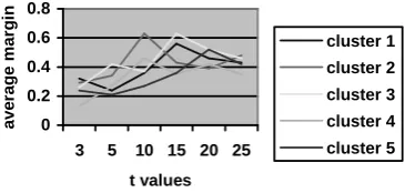
For sentence classification, we need to estimate the parameter t. We randomly chose 5 document clusters and one manual summary from the four. Fig. 7 shows the change of the average margin over all the top 40% sentences in a cluster with t varying from 3 to 25.

0 0.2 0.4 0.6 0.8

3 5 10 15 20 25 t values

a

v

e

ra

g

e

m

a

rg

in

cluster 1 cluster 2 cluster 3 cluster 4 cluster 5

Fig. 7. Average margin and t

estimate the best t for each cluster.

After estimation of t, EM was used to estimate the membership probabilities. Table 1 gives the average pointwise entropy for top 10% to top 100% sentences in each cluster, where sentences were ordered by their membership probabilities. The values were averaged over 20 runs, and for each run, 10 document clusters and one summary were randomly selected, and the entropy was averaged over the summaries.

Sentences E_Semi E_SVM Significance

10% 0.23 0.22 ~

20% 0.26 0.27 ~

30% 0.32 0.43 *

40% 0.35 0.49 **

50% 0.42 0.51 *

60% 0.46 0.55 *

70% 0.48 0.57 *

80% 0.59 0.62 ~

90% 0.65 0.69 ~

100% 0.70 0.73 ~

Table 1. Entropy of classification result

In Table 1, the column E_Semi shows entropies of the semi-supervised classification. It indicates that the entropy increases as more sentences are considered. This is not surprising since the sentences are ordered by their membership probabilities in a cluster, which can be seen as a kind of measure for closeness between sentences and cluster centroids, and the boundaries between clusters become dim with more sentences considered.

To compare the performance between this semi-supervised classification and a standard supervised method like Support Vector Machines (SVM), Table 1 also lists the average entropy of a SVM (E_SVM) over the runs. Similarly, we found that the entropy also increases as sentences increase. Table 2 also gives the significance sign over the runs, where *, ** and ~ represent p-values <=0.01, (0.01, 0.05] and >0.05, and indicate that the entropy of the semi-supervised

classification is lower, significantly lower, or almost the same as that of SVM respectively. Table 1 demonstrates that when the top 10% or 20% sentences are considered, the performance between the two algorithms shows no difference. The reason may be that these top sentences are closer to cluster centroids in both cases, and the cluster boundaries in both algorithms are clear in terms of these sentences.

For the top 30% sentences, the entropy for semi-supervised classification is lower than that for a SVM, and for the top 40%, the difference becomes significantly lower. The reason may go to the substantial assumptions behind the two algorithms. SVM, based on local comparison, is successful only when more labeled data is available. With only one sentence labeled as in our case, the semi-supervised method, based on global distribution, makes use of a large amount of unlabeled data to reveal the underlying manifold structure. Thus, the performance is much better than that of a SVM when more sentences are considered.

For the top 50% to 70% sentences, E_Semi is still lower, but not by much. The reason may be that some noisy documents are starting to be included. For the top 80% to 100% sentences, the performance shows no difference again. The reason may be that the lower ranking sentences may belong to other classes than those represented by summary sentences, and with these sentences included, the cluster boundaries become unclear in both cases.

6.4 Evaluation of Ordering

some sentences in the documents, we also tried to combine two or three consecutive sentences into one, and tested their ordering performance (τ_2 and τ_3) respectively.

τ HO MO PO τ_1 0.42 0.31 0.33 τ_2 0.33 0.26 0.29 τ_3 0.27 0.21 0.25 Table 2. τ scores for HO, MO and PO

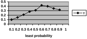
Table 2 indicates that the combination of sentences harms the performance. To see why, we checked the classification results, and found that the pointwise entropies for two and three sentence combinations (for the top 40% sentence in each cluster) increase 12.4% and 18.2% respectively. This means that the cluster structure becomes less clear with two or three sentence combinations, which would lead to less similar sentences being clustered with summary sentences. This result also suggests that if the summary sentence subsumes multiple sentences in the documents, they tend to be not consecutive. Fig. 8 shows change of τ scores with different number of sentences used for ordering, where x axis denotes top (1-x)*100% sentences in each cluster. The score was averaged over 20 runs, and for each run, 10 summaries were randomly selected and evaluated.

0 0.1 0.2 0.3 0.4 0.5

0.1 0.2 0.3 0.4 0.5 0.6 0.7 0.8 0.9 1 least probability

τ

Fig. 8. τ scores and number of sentences

Fig. 8 indicates that with fewer sentences (x >=0.7) used for ordering, the performance decreases. The reason may be that with fewer and fewer sentences used, the result is deficient

training data for the ordering. On the other hand, with more sentences used (x <0.6), the performance also decreases. The reason may be that as more sentences are used, the noisy sentences could dominate the ordering. That’s why we considered only the top 40% sentences in each cluster as training data for sentence reordering here.

As an example, the following is a summary for a cluster of documents about Central American storms, in which the ordering is given manually.

1) A category 5 storm, Hurricane Mitch roared across the northwest

Caribbean with 180 mph winds across a 350-mile front that

devastated the mainland and islands of Central America.

2) Although the force of the storm diminished, at least 8,000 people

died from wind, waves and flood damage.

3) The greatest losses were in Honduras where some 6,076 people

perished.

4) Around 2,000 people were killed in Nicaragua, 239 in El Salvador,

194 in Guatemala, seven in Costa Rica and six in Mexico.

5) At least 569,000 people were homeless across Central America.

6) Aid was sent from many sources (European Union, the UN, US

and Mexico).

7) Relief efforts are hampered by extensive damage.

4th position. This suggests that consideration of selection history does in fact help to group those related sentences more closely, although sentence 2 was ranked lower than expected in the example.

In MO, we found sentence 2 was put immediately behind sentence 3. The reason was that, after sentence 1 and 3 were selected, the in-edges of the node representing cluster 2 became 0 in the cluster directed graph, and its in-out edge difference became the biggest among all nodes in the graph, so it was chosen. For similar reasons, sentence 6 was put behind sentence 2. This suggests that it may be difficult to consider the selection history in MO, since its selection is mainly based on the current status of clusters.

6. Conclusion and Future Work

In this paper, we propose a sentence ordering method for multi-document summarization based on semi-supervised classification and historical ordering. For sentence classification, the semi-supervised classification groups sentences based on their global distribution, rather than on local comparisons. Thus, even with a small amount of labeled data (just 1 labeled example in our case) we nevertheless ensure good performance for sentence classification.

For sentence ordering, we propose a kind of history-based ordering strategy, which determines the next selection based on the whole selection history, rather than the most recent single selection in probabilistic ordering, which could result in topic bias, or in-out difference in MO, which could result in topic disruption. In this work, we mainly use sentence-level information, including sentence similarity and sentence order, etc. In future, we may explore the role of term-level or word-level features, e.g., proper nouns, in the ordering of summary sentences. To make summaries more coherent and readable, we may also need to discover how to detect and control topic movement automatic

summaries. One specific task is how to generate co-reference among sentences in summaries. In addition, we will also try other semi-supervised classification methods, and other evaluation metrics, etc.

Reference

Barzilay, R N. Elhadad, and K. McKeown. 2002.

Inferring strategies for sentence ordering in

multidocument news summarization. Journal of

Artificial Intelligence Research, 17:35–55.

Bollegala D. Okazaki, N. Ishizuka, M. 2005. A

Machine Learning Approach to Sentence Ordering

for Multidocument Summarization, in Proceedings

of IJCNLP.

Dash M. and H. Liu, (2000) Unsupervised feature

selection, proceedings of PAKDD.

Filatova, E. & Hovy, E. (2001) Assigning time-stamps

to event-clauses. In Proceedings of AACL/EACL

workshop on Temporal and Spatial Information

Processing.

Lapata, M. 2003. Probabilistic text structuring: Experiments with sentence ordering. In Proceedings

of the annual meeting of ACL 545–552.

Lin, J. 1991. Divergence Measures Based on the

Shannon Entropy. IEEE Transactions on

Information Theory, 37:1, 145–150.

McKeown K., Barzilay R. Evans D., Hatzivassiloglou

V., Kan M., Schiffman B., &Teufel, S. (2001).

Columbia multi-document summarization:

Approach and evaluation. In Proceedings of DUC. Reiter, Ehud and Robert Dale. 2000. Building Natural

Language Generation Systems. Cambridge

University Press, Cambridge.

Szummer M. and T. Jaakkola. (2001) Partially labeled

classification with markov random walks. NIPS14. Tishby, N, Slonim, N. (2000) Data clustering by

Markovian relaxation and the Information

Bottleneck Method. NIPS 13.

Zhu, X., Ghahramani, Z., & Lafferty, J. (2003) Semi-Supervised Learning Using Gaussian Fields

and Harmonic Functions. ICML-2003.

Zhou D., Bousquet, O., Lal, T.N., Weston J. &